CS180: Introduction to Computer Vision & Computation Photography

Project 2

Fun with Filters and Frequencies

Clara Hung

Project Overview

Project 2 is a big mish-mosh of different sub-projects that explores how to manipulate image frequencies. By the end of the project, we should be able to have some fun with multi-resolution blending!

Part 1: Fun with Filters

1.1 Finite Difference Operator

Approach

One way to implement an edge-detector, or a high-pass filter (HPF), is to take the derivative of an image. However, how does one take a derivative (a continuous operation) over a discrete space that is an image? Here comes the Finite Difference Operator (FDO) to the rescume! The FDO is a simple filter that approximates the gradient of an image, and we define a FDO in each direction in the image (x, y):

$$D_x = \begin{bmatrix} -1 & 1 \end{bmatrix}$$

$$D_y = \begin{bmatrix} -1 \\ 1 \end{bmatrix}$$

To obtain the partial derivative of the image (I) in both the x and y directions, we convolve the image with the FDOs. (Why can't we take a multi-dimensional derivative simultaneously? Beats me -- ask the math department!)

$$\frac{\partial I}{\partial x} = I \ast D_x$$

$$\frac{\partial I}{\partial y} = I \ast D_y$$

The magnitude of the gradient can be calculated by taking the square root of the sum of the squares of the partial derivatives:

$$\text{Gradient Magnitude} = \| \nabla f \| = \sqrt{(\frac{\partial I}{\partial x})^2 + (\frac{\partial I}{\partial y})^2}$$

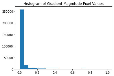
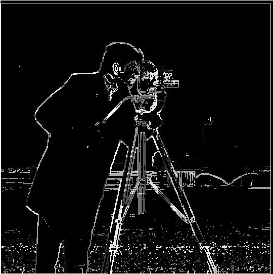
To obtain an edge image, we can binarize the gradient magnitude by choosing a threshold and setting all values below the threshold to be zero and above to be 1. In the images below, I set the threshold to be 0.1, chosen after plotting a histogram of the gradient magnitude's pixel values. Most of the values will be 0 or noise. Notice how, even with the 0.1 threshold, the edge image is still quite noisy! We can still see some specs on the grass, and we don't want that!

Results

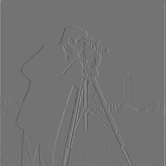
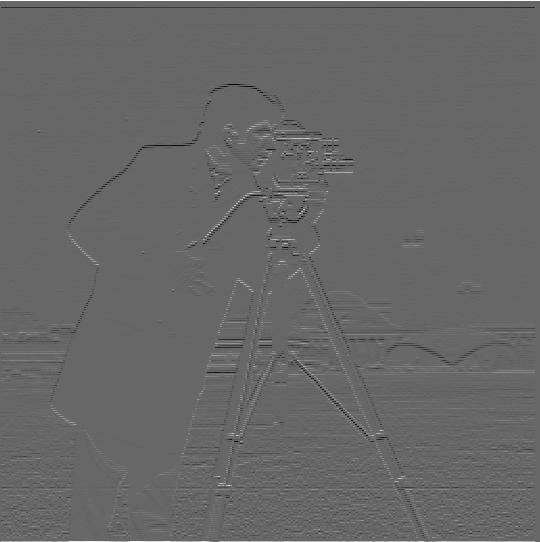
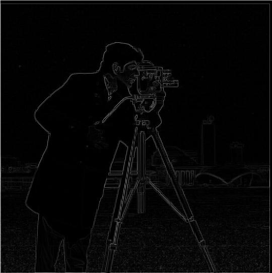
1.2 Derivative of a Gaussian (DoG) Filter

So, how should we get rid of noise? Since noise is a high-frequency component, let's low-pass filter (LPF) it first with a Gaussian! For this, we can use the associativity and commutivity of the convolution to have two implementations of the same filter: taking the derivative of a gaussian-filtered image is the same as convolving the image with a derivative-of-gaussian (DoG) filter!

$$\frac{\partial}{\partial x} (I \ast G) = I \ast (\frac{\partial}{\partial x} G)$$

For my implementation, I used cv2.getGaussianKernel with kernel_size = 10 and sigma=kernel_size/6. This took a little bit of fine-tuning to get right as sometimes, when the kernel size is too small, the DoG doesn't filter properly. Here are some results of the gradient magnitude, normalized to [0, 1]:

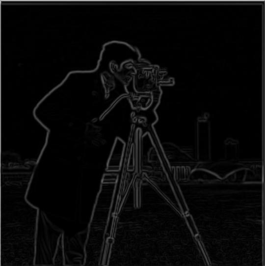
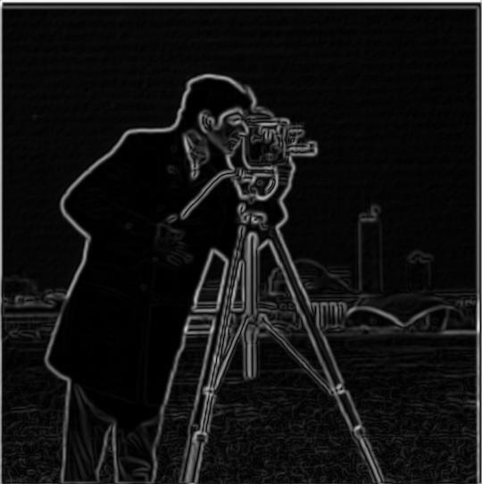
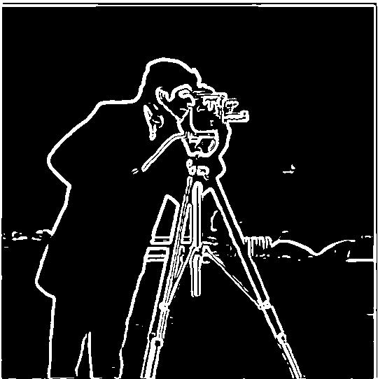
For these images, using the same threshold of 0.1, we can clearly see that the edges are significantly cleaner than the FDO without the LPF. Additionally, there are no longer (or if there are, very few) high frequency componenets on the grassy area. The lines are thicker, but that's likely because the LPF smooths the edges out. When we compare the images from the two methods, it appears that they are nearly identical, sans some intensity differences that may due to implementation and bit-depth inaccuracies. For reference, here are my DoG filters! They look super blurry because they're blown up from a small 10x10 kernel.

Part 2: Fun with Frequencies

2.1 Image "Sharpening"

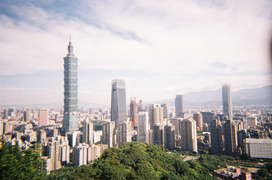
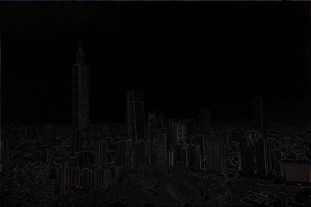
Image sharpening is a technique that enhances the edges of an image by accentuating the high-frequency components. One way to do this is to subtract the low-pass filtered image from the original image. This is equivalent to adding the high-pass filtered image to the original image. Mathematically, we define it as follows:

$$\text{Sharpened Image} = \text{Original Image} + \alpha(\text{Original Image} - \text{Low-pass Filtered Image})$$

Where \(\alpha\) is a multiplier that defines how much the image should be sharpened. Below, the \(\sigma, k, \alpha\) values of each image are included next to the sharpened image.

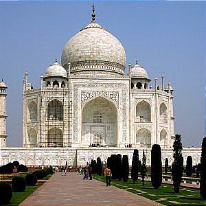
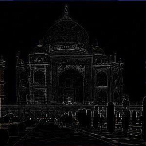
I took this film photo myself!

For evaluation, let's test a sharp image, blur it, then try to sharpen it again.

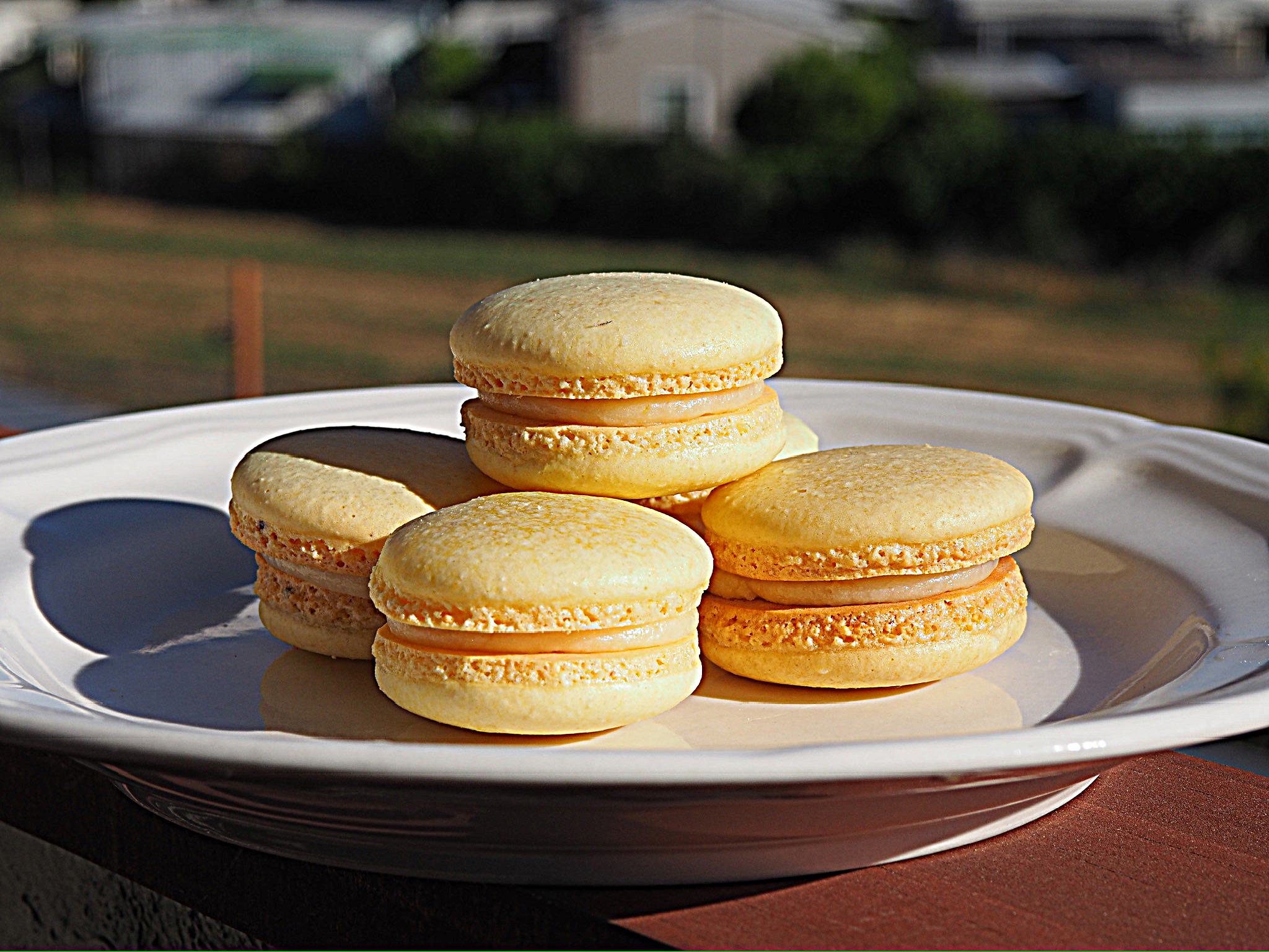
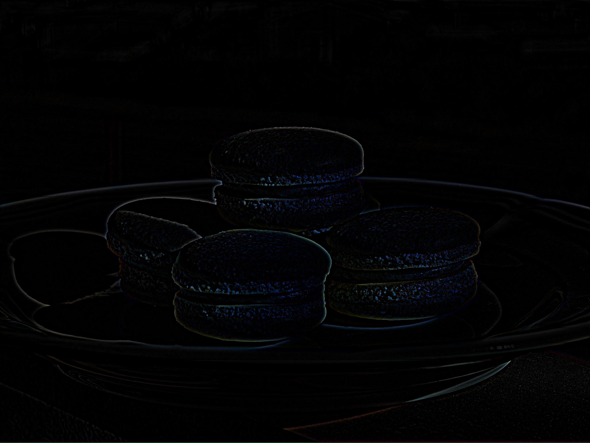
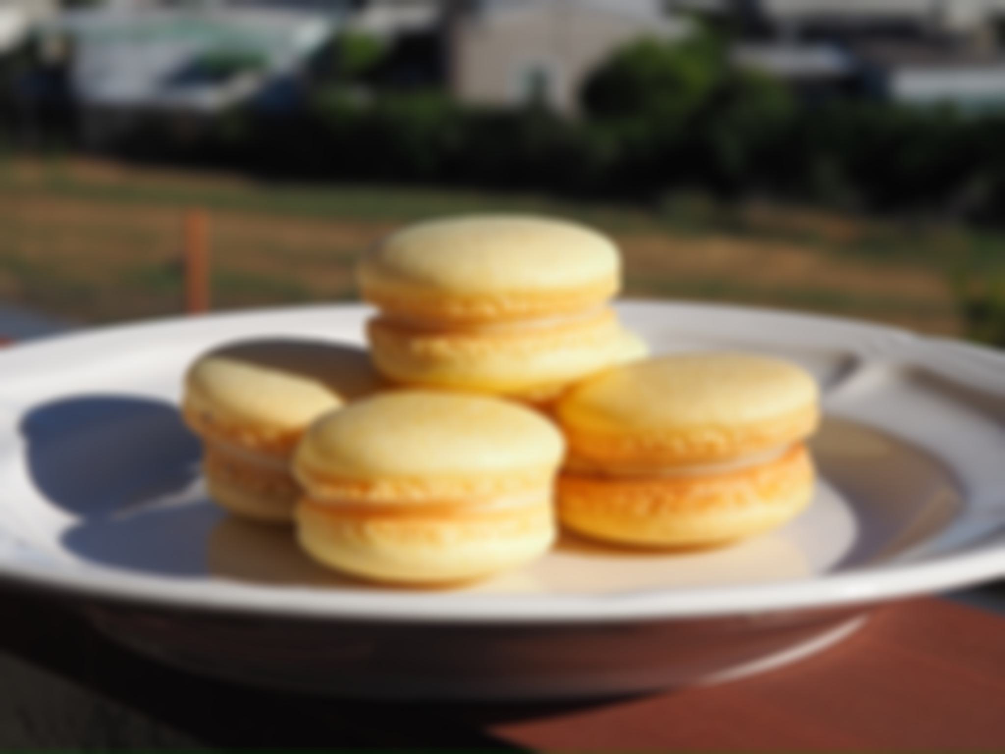
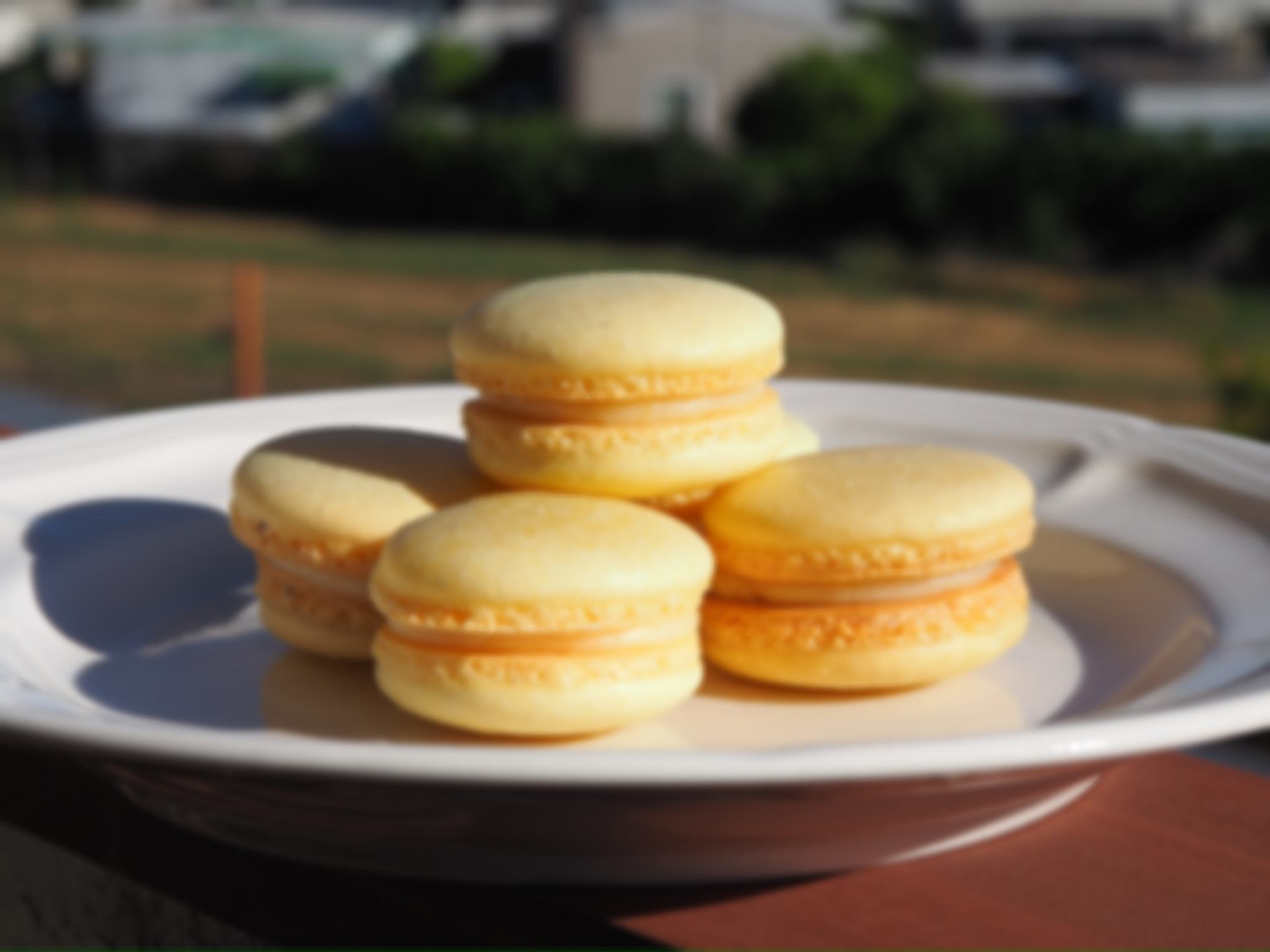
From the images above, it is clear that when we attempt to sharpen our blurred macarons with its own details, the images become slightly sharper compared to the original blurred macarons, but not by much, whereas when we sharpened the blurred image with details from the original filter, we do get a sharper image back if we turn up the \(\alpha\) factor. This is likely because when we first LPF the macarons to get the blurred image, a lot of the high frequency content is already filtered out. Thus, we cannot add more high frequency content back (remember Babak's core tenant of LTI systems: no new frequencies!!!). However, we can manually add the high frequency content back by using the mask of the original image. This poses an interesting problem for deblurring applications: can we deblur without priors?

2.2 Hybrid Images

Next, we can try hybridizing images! For this section, we will superimpose two images together: one that is LPF-ed, leaving only LF components; one that is HPF-ed, leaving only HF components. The idea here is that when we look at the image from far away, our eyes are accustomed to seeing LF content, whereas if we look up close, we are used to seeing HF content. For Derek and Nutmeg, I aligned using the sparkle in their eye. I used a larger gaussian kernel (15) and a larger sigma for greater smoothing (10). I saved these images as grayscale since, when you choose images that have different intensities and color profiles, the hybrid images look a bit wacky. Images worked best when I had a larger kernel, with a greater \(\sigma\( for the HPF and smaller for the LPF. As a side note, I had to make sure my type conversions were correct (clip 0-255,then normalize) for when saving as gray scale, the images must be in uint8.

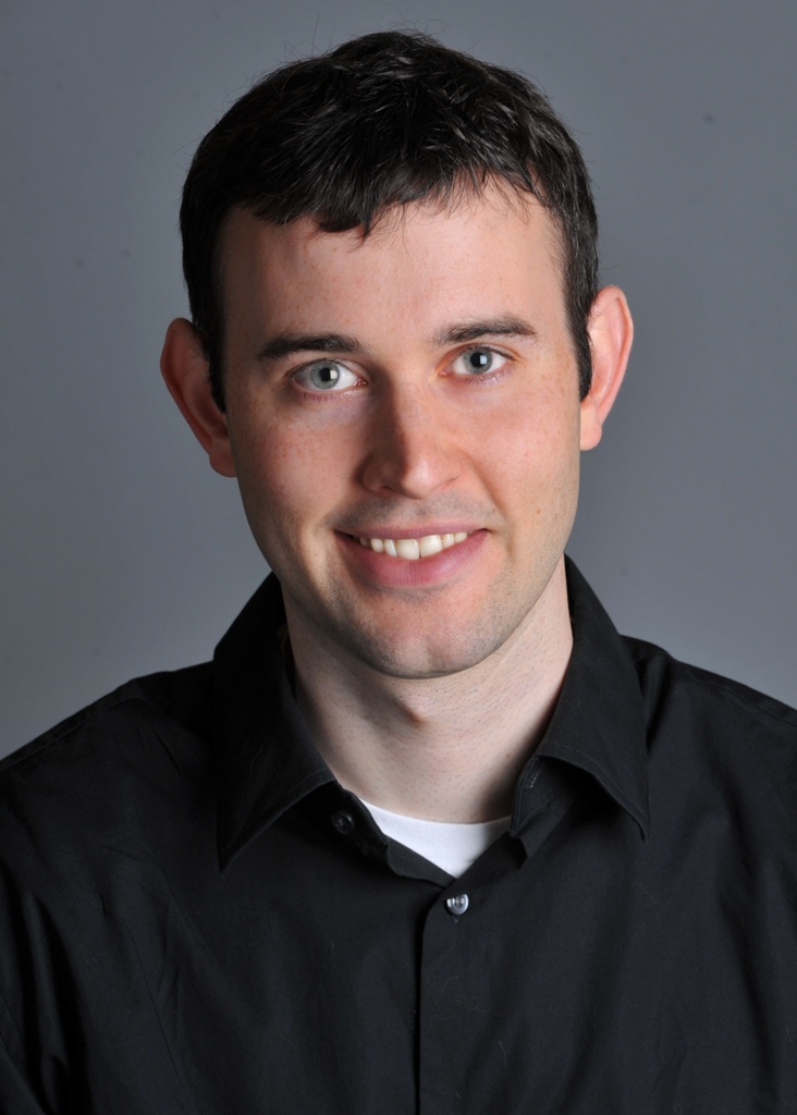
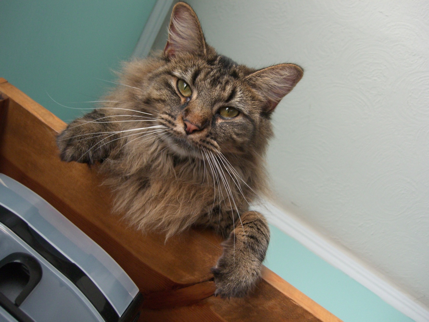
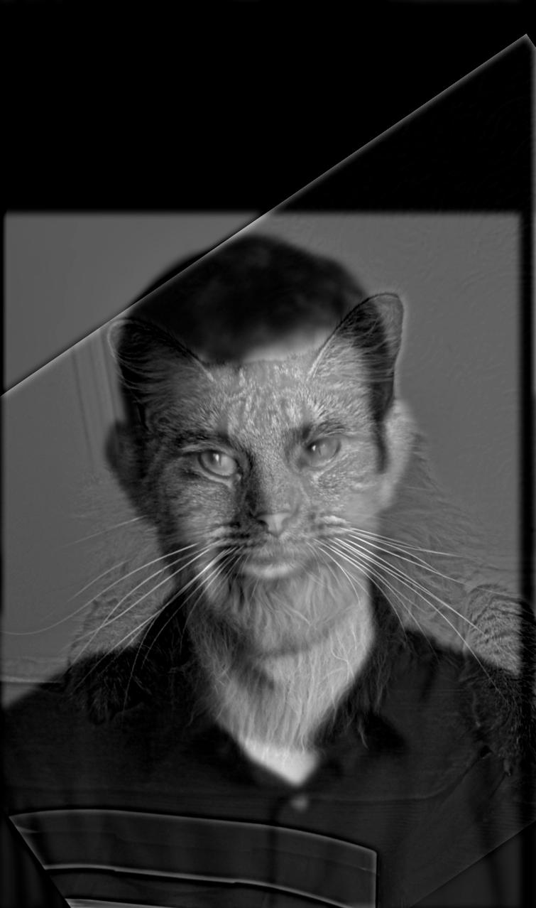
Here are a couple other I tried! This has great applications for biomimicry!

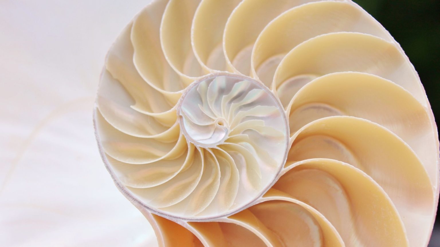
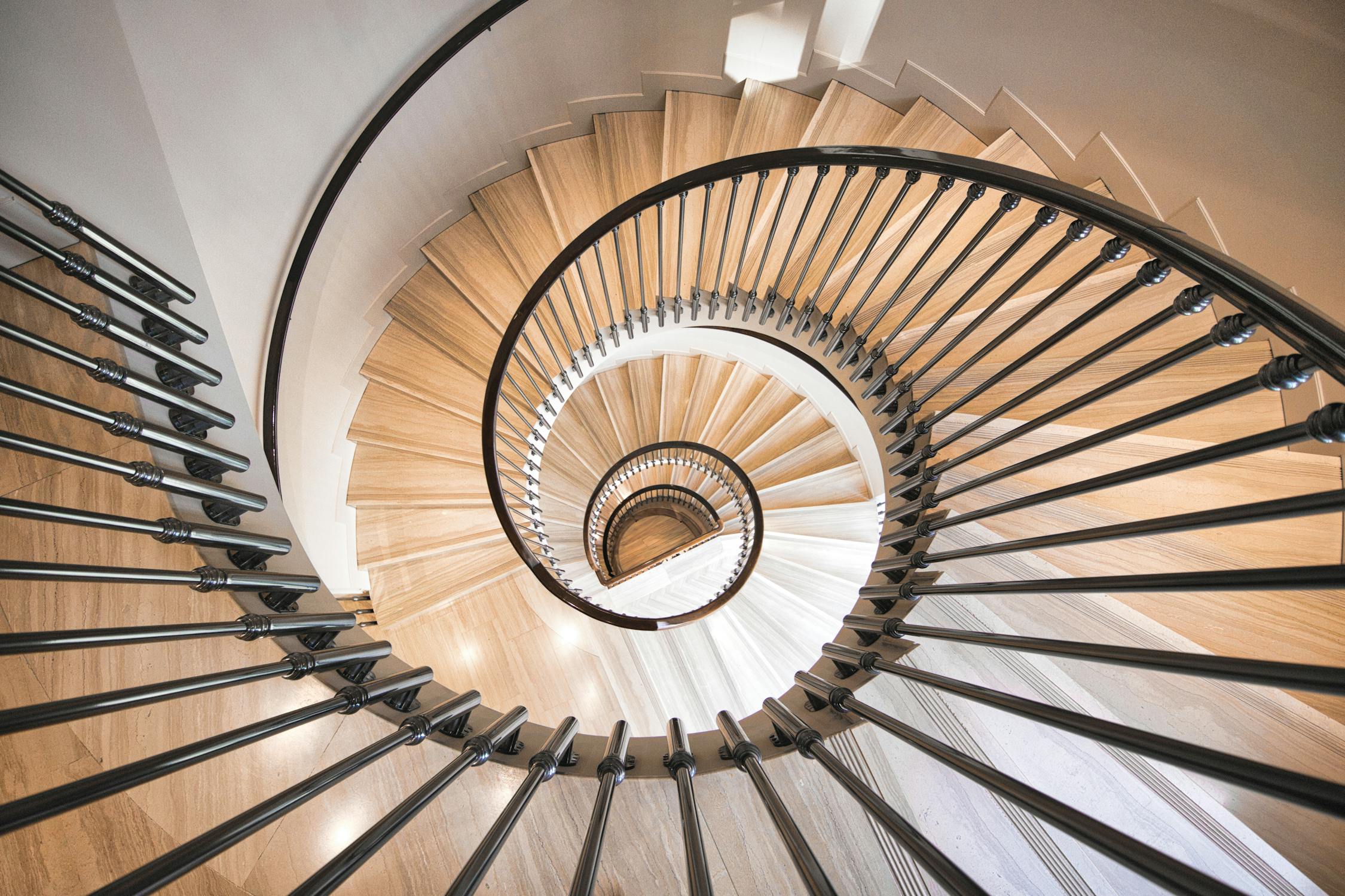
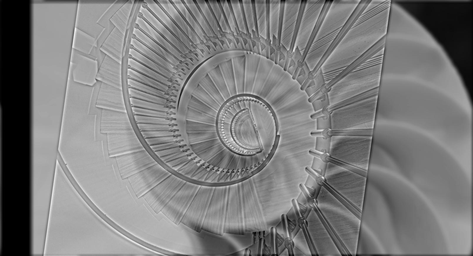
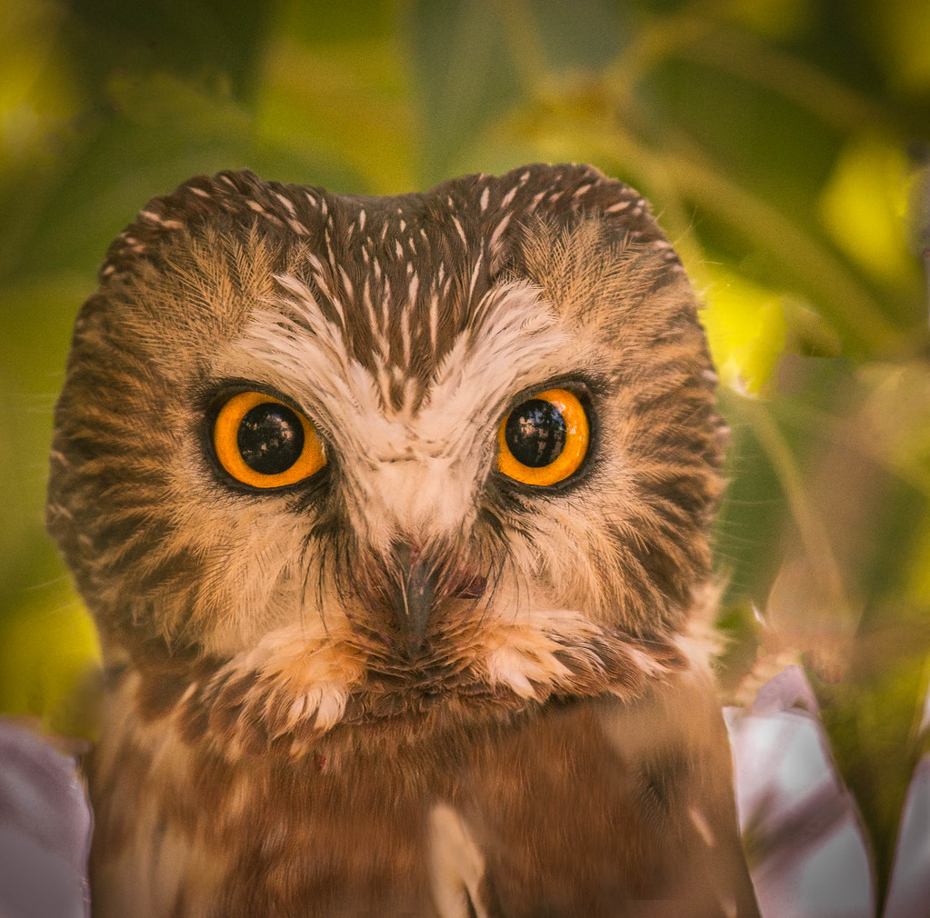
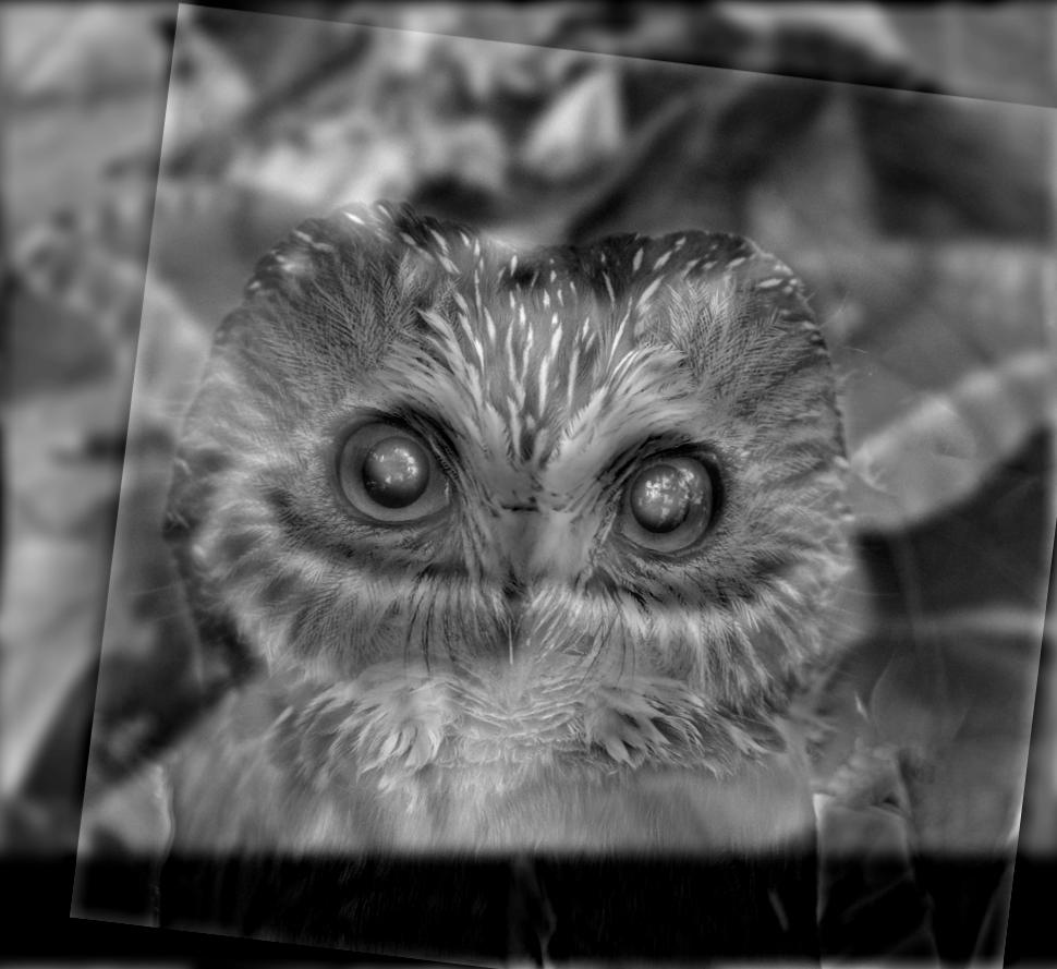
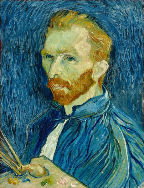
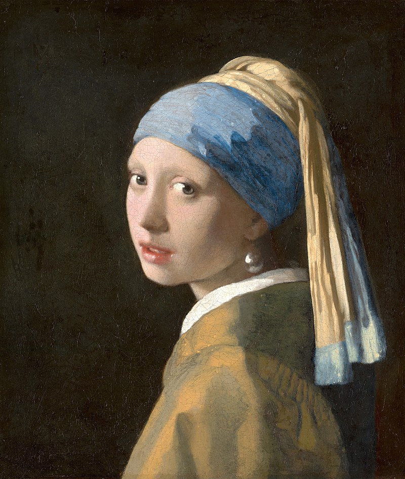
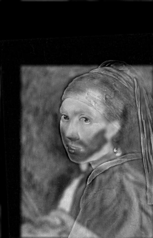
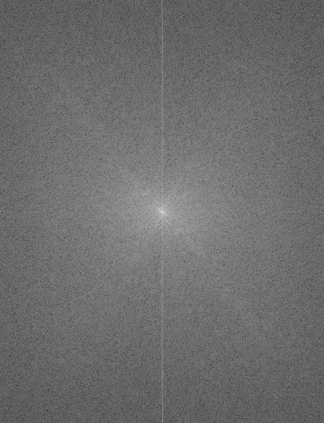
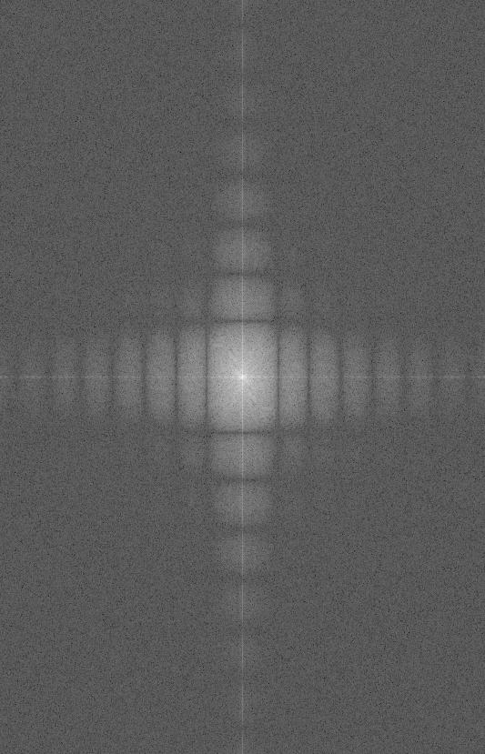
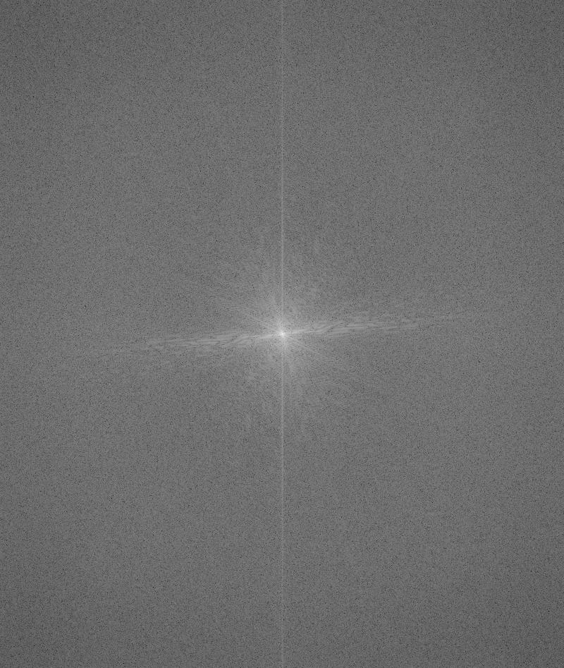
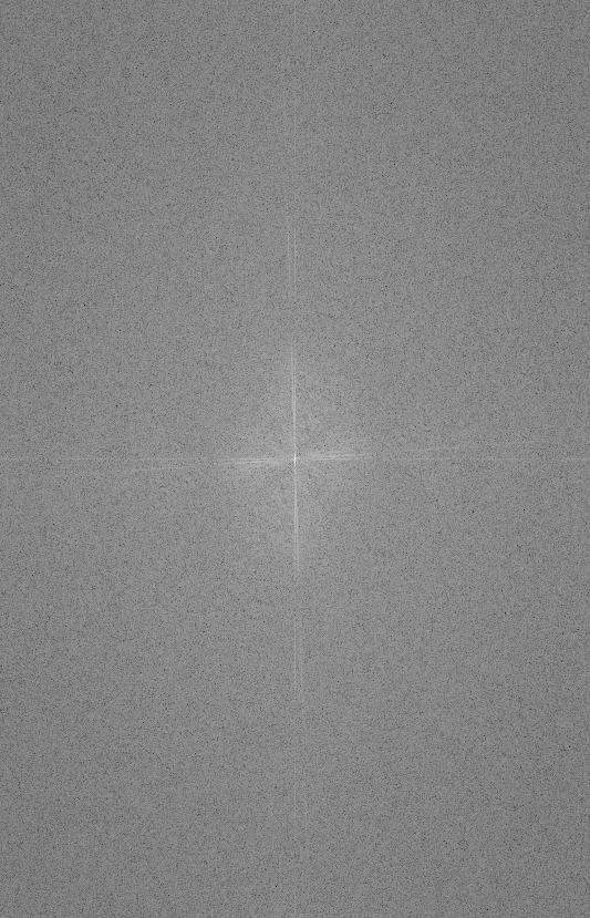
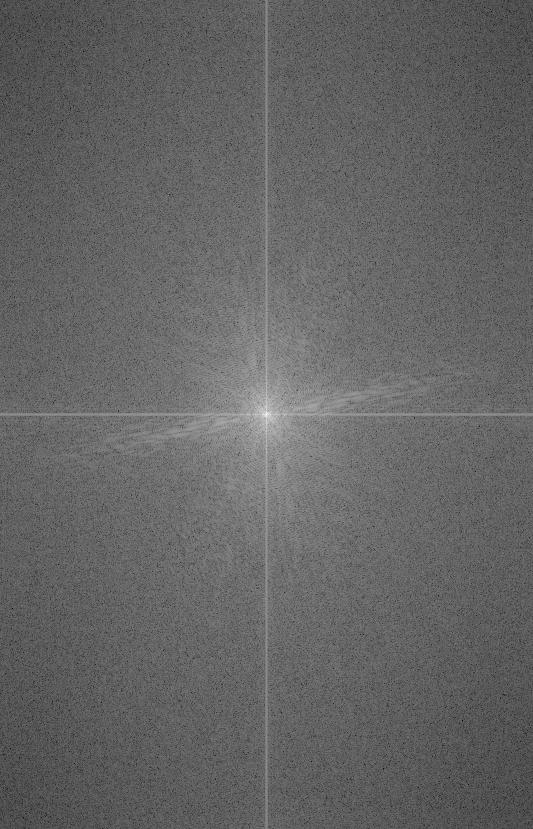
Here's a Fourier analysis of the paintings. The difference in sizing is a result of the alignment. You can notice there are some sidelobes in the Filtered Van Gogh. That may be a result of a windowing operation, perhaps in the alignment, or that our LPF was far too tight.

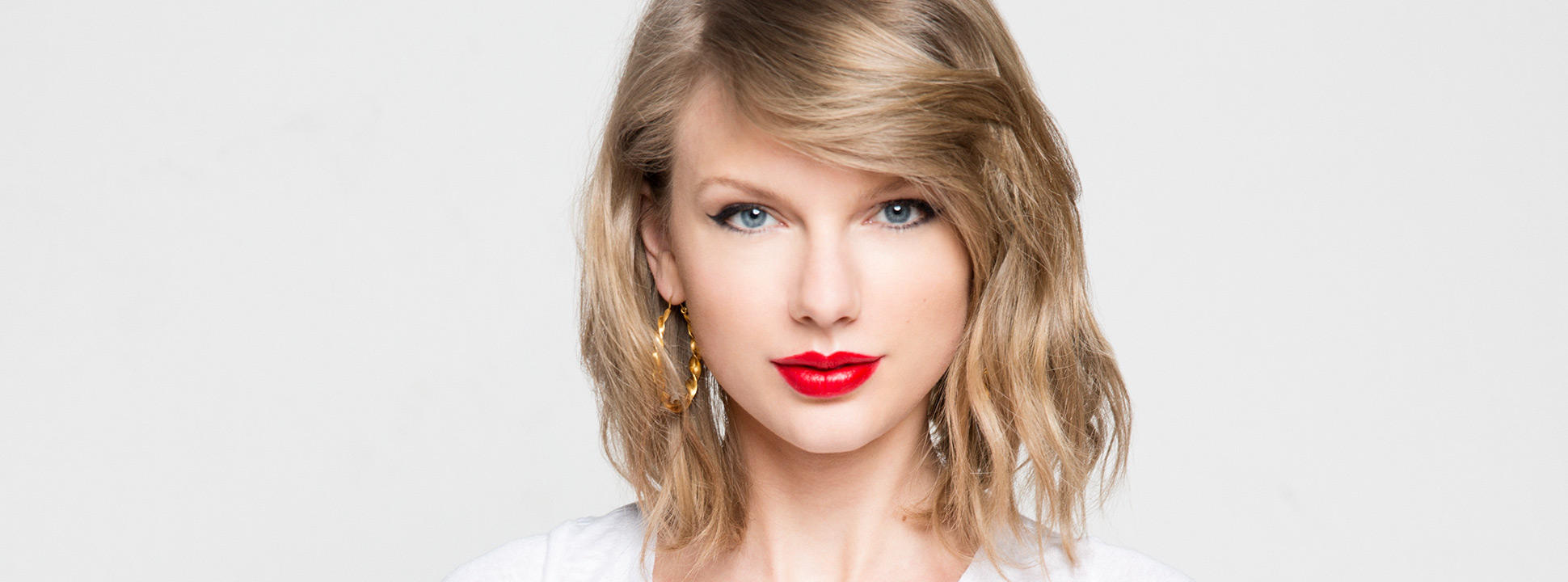
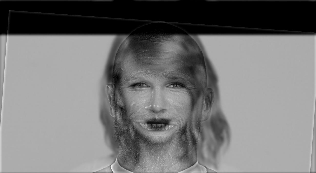
Failure cases! Sometimes this hybrid imaging doesn't really work! I think it is because Taylor and Travis don't really have comparable face shapes, and if they do, Travis's beard gets in the way. His mouth is also a bit large, so I don't think the results look nearly as good as the previous ones. In this case, I also think I need to increase the \(\sigma\) of Travis since I think his HF components need to be accentuated. You can see Taylor more clearly than Travis.

Multi-Resolution Blending and the Oraple Journey

2.3 Gaussian and Laplacian Stacks

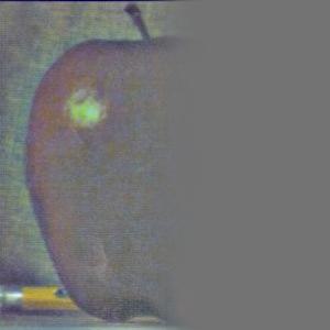
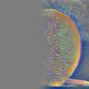
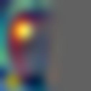
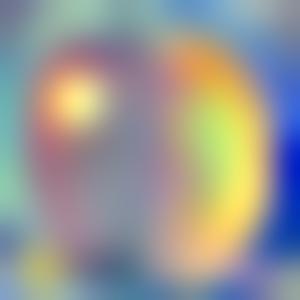
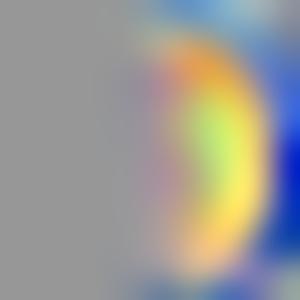
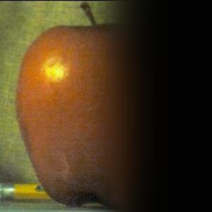
Here are the results of my Laplacian stacks with a binary half-half mask for creating the Oraple! Level 0 is the highest frequency layer, Level 2 medium frequencies, and Level 4 the lowest frequency layer! Additionally for the blending, I found that it was helpful to pass my mask through a LPF first to smooth out the sharp transitions. For all of the following blends, my parameters were as follows: \(\text{depth} = 5, \sigma = 16, k = 6\sigma + 1\). Why the formula for the kernel size? I didn't want to manually guess and check kernel sizes, so I looked online for general heuristics on how kernel size should be determined.

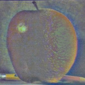
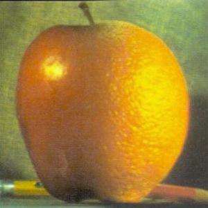
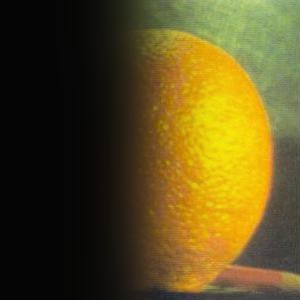
2.4 Multi-Resolution Blending: the Oraple's final Journey!

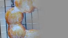
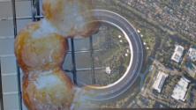
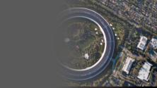
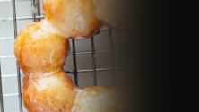
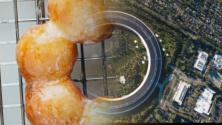
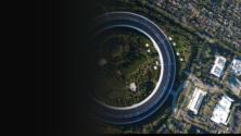
People often say that Apple Park (AP) looks like a doughnut... does it? For this, I had to use the alignment starter code to align the donut and AP. It was hard to find images that had similar lighting.

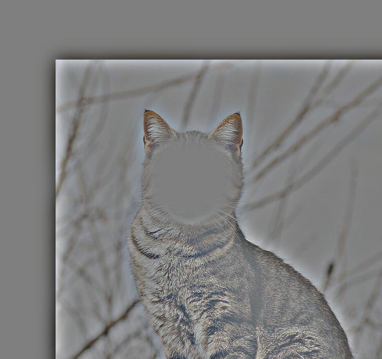
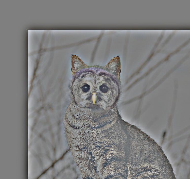
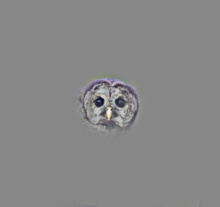
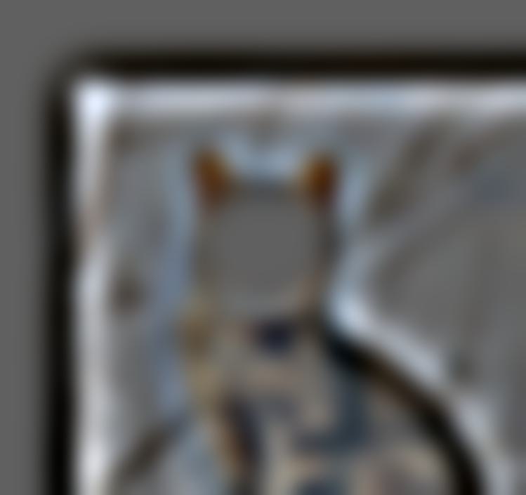
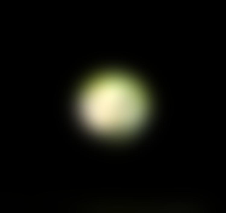
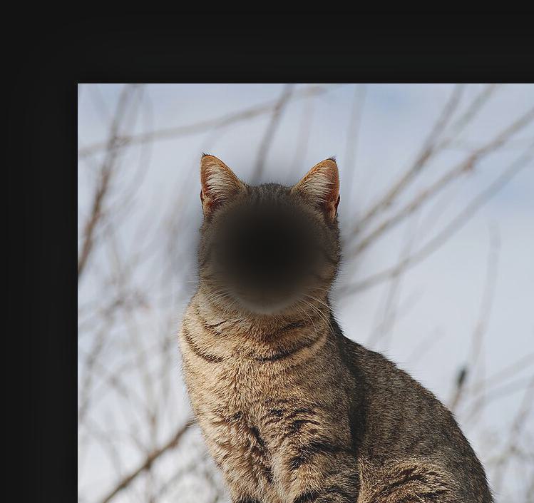
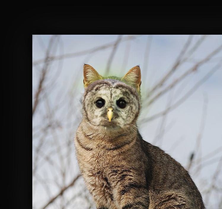
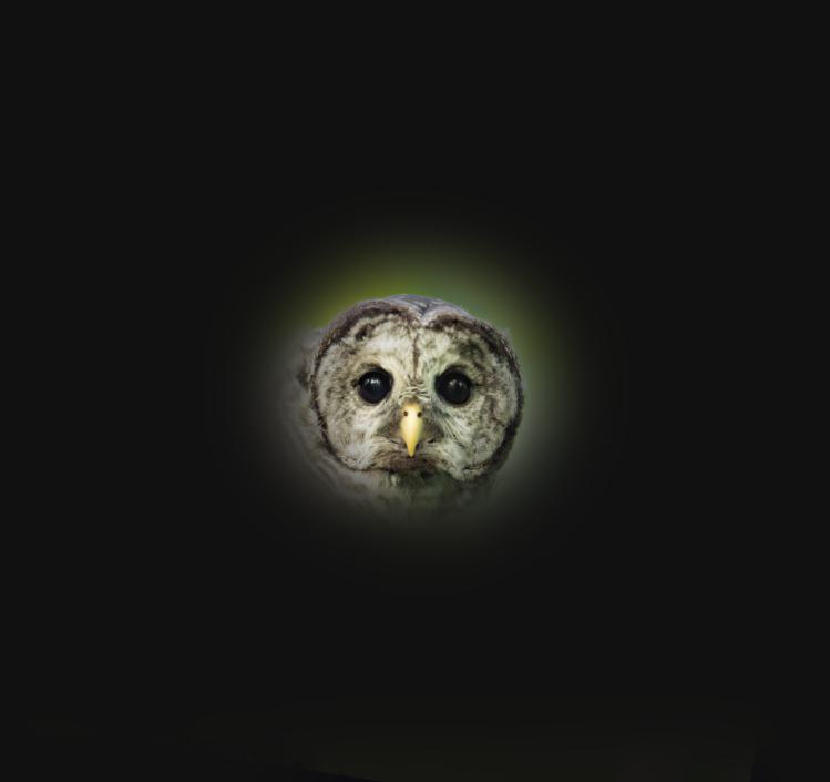
An irregular mask, you say? This was inspired by my friend Viraj who wanted a catowl in the spirit of the catowl reddit page. I first aligned the cat and owl using the given starter code. Then, I used the aligned images to create my mask by positioning a circle on keynote to cover the owl's head. I took a screenshot of this and loaded it in as a numpy array. (Someone should teach me how to use Photoshop.)