CS180: Introduction to Computer Vision & Computation Photography

Project 4

Stitching Photo Mosaics

Clara Hung

Project Overview

The goal of this project is to get hands-on experience with different methods of image warping applied to image mosaicing. Trhough this, we will create an image mosaic by first taking our own photographs, then register, projective warp, resample, and composite images. Then, we will automate correspondence-finding so we can generate panoramas automatically. As for Part A, it's homography time!

1. Shooting Photos

See photos below!

2. Recover Homographies

As a refresher, here is how we can solve for the homography matrix given a set of points! A homography performs the transformation \(p' = Hp\), where \(p'\) is the original set of points and \text{p'} are the points you are trying to warp to. If we have a homography matrix:

$$ H = \begin{pmatrix} h_{1} & h_{2} & h_{3} \\ h_{4} & h_{5} & h_{6} \\ h_{7} & h_{8} & 1 \end{pmatrix} $$

and a set of points:

$$ \begin{pmatrix} x_{1} & y_{1} & 1 \\ x_{2} & y_{2} & 1 \\ x_{3} & y_{3} & 1 \\ x_{4} & y_{4} & 1 \end{pmatrix} $$

We can solve for the homography matrix by setting up the following equations and solving via least squares:

$$ \begin{bmatrix} x_1 & y_1 & 1 & 0 & 0 & 0 & -x'_1 x_1 & -x'_1 y_1 \\ 0 & 0 & 0 & x_1 & y_1 & 1 & -y'_1 x_1 & -y'_1 y_1 \\ x_2 & y_2 & 1 & 0 & 0 & 0 & -x'_2 x_2 & -x'_2 y_2 \\ 0 & 0 & 0 & x_2 & y_2 & 1 & -y'_2 x_2 & -y'_2 y_2 \\ & & & & \vdots & & & \\ \end{bmatrix} \begin{bmatrix} h_1 \\ h_2 \\ h_3 \\ h_4 \\ h_5 \\ h_6 \\ h_7 \\ h_8 \end{bmatrix} = \begin{bmatrix} x'_1 \\ y'_1 \\ x'_2 \\ y'_2 \\ \vdots \end{bmatrix} $$

In the end, we get:

\[ \begin{bmatrix} x' \\ y' \\ w \end{bmatrix} = \begin{bmatrix} h_1 & h_2 & h_3 \\ h_4 & h_5 & h_6 \\ h_7 & h_8 & 1 \end{bmatrix} \begin{bmatrix} x \\ y \\ 1 \end{bmatrix} \]

which becomes:

\[ \begin{bmatrix} \frac{x'}{w} \\ \frac{y'}{w} \end{bmatrix} \]

For this project, I used this tool to help me define each of the correspondance points in the images.

3. Image Rectification

A simple way to test if our homography works is by rectifying an image. Say I had a photo of a sign viewed from an angle:

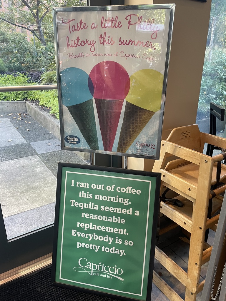
Coffee Sign Viewed from an Angle

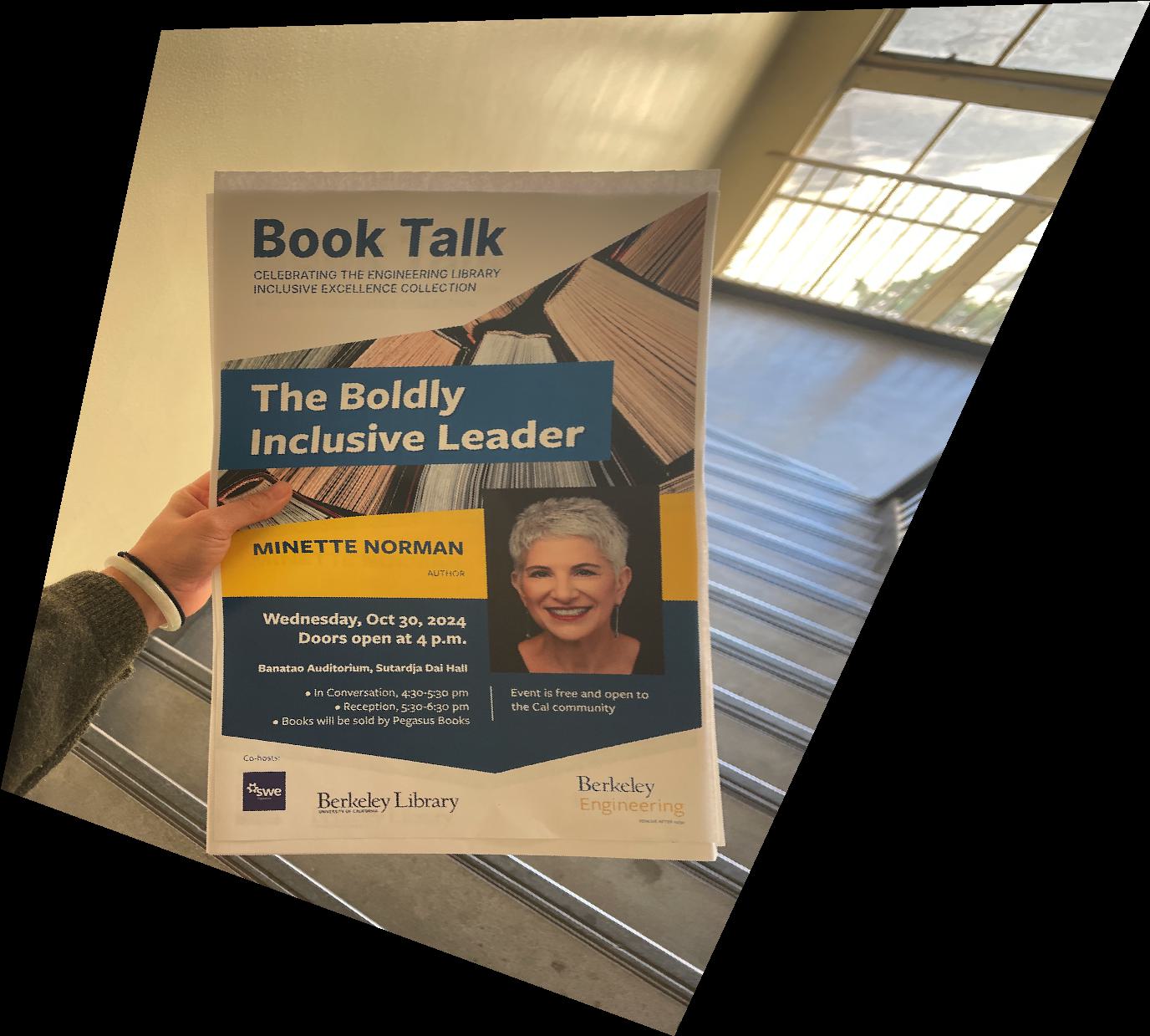
But I want to view it head-on. I can compute the homography transform from the coordinate system of the original image to the coordinate system of a rectified image. Now, I will be able to see the sign as if I were looking at it directly!

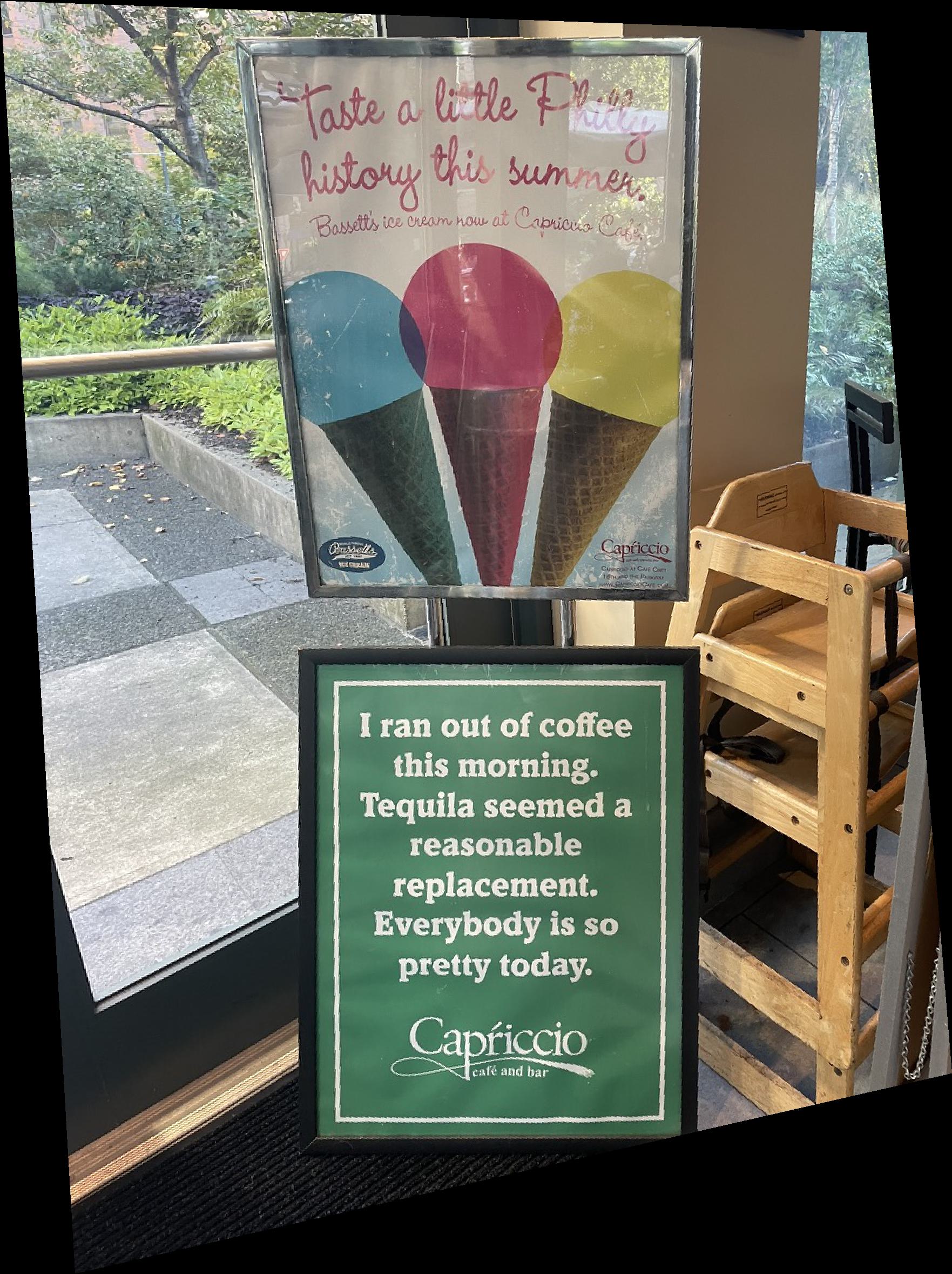
Rectified Coffee Sign

Here's another example applied to the license plate "ICHBIN". The actual license plate is small, but you can see how the license plate is now facing us.

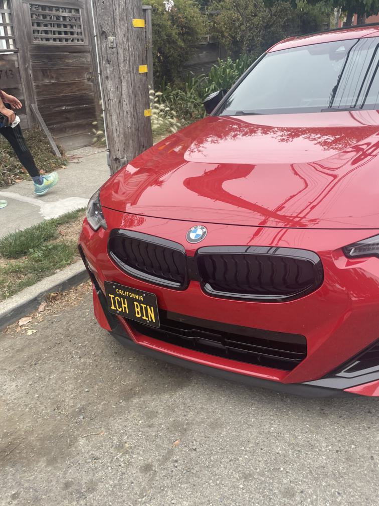
License Plate "ICHBIN"

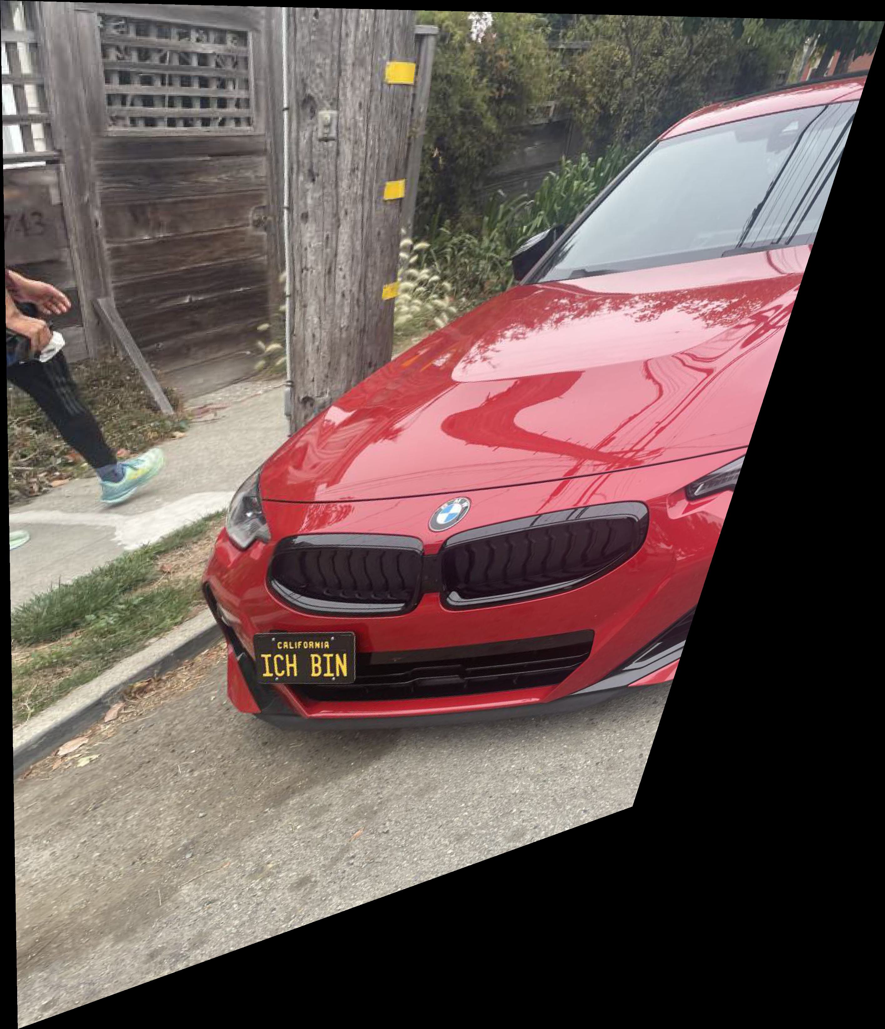
Rectified "ICHBIN"

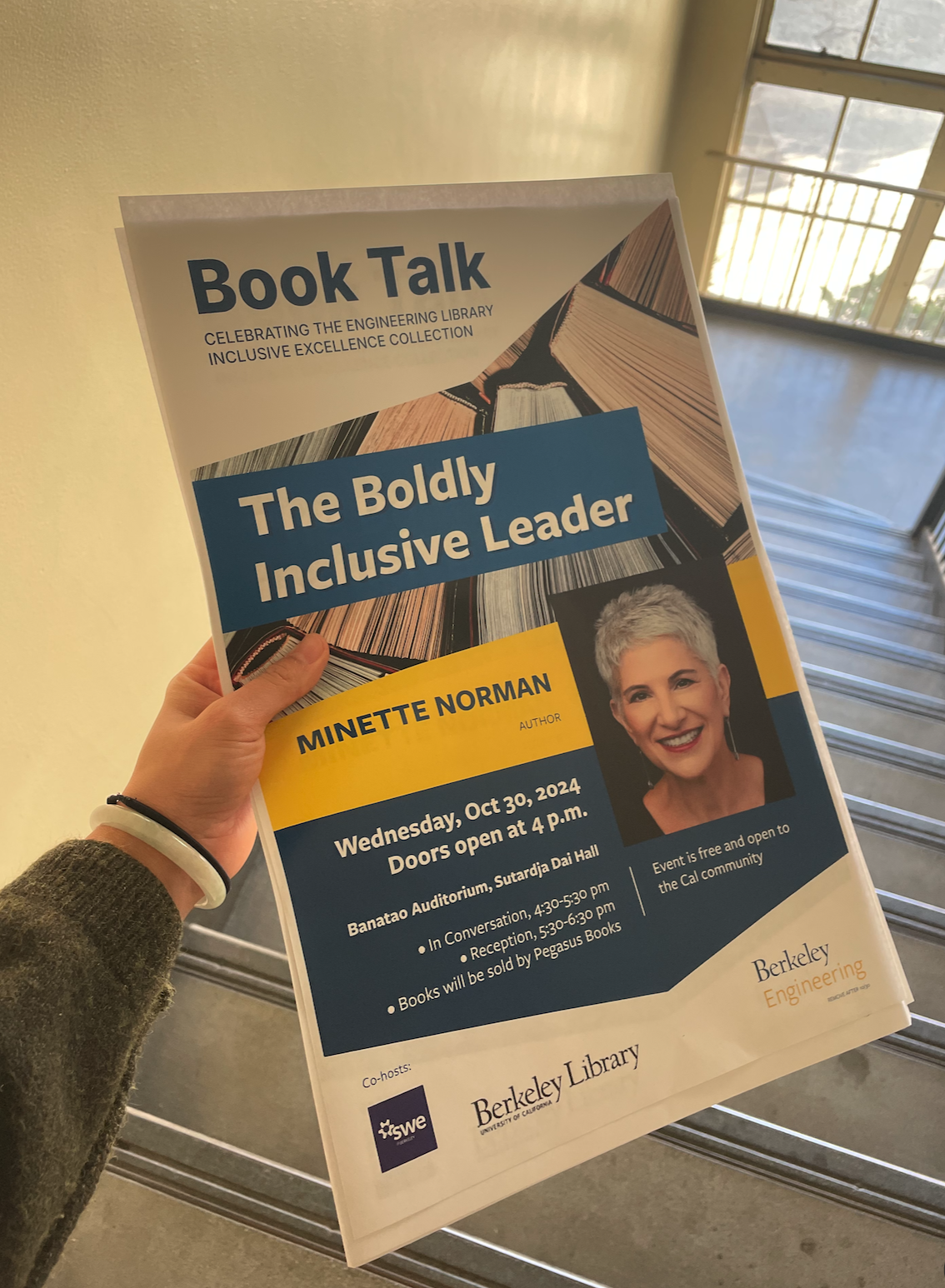
And another example applied to this book talk poster. Fun fact, I will be moderating this talk! You should come!

Book Talk

Rectified Booktalk

A couple things I learned here:

• Make sure the corners of the surface you're trying to rectify are in the same order as your rectified corners.
• Remember to choose your points such that, when you use polygon to recover your bounding box, the polygon's lines don't cross. That is, choose the points in an order such that the polygon has as large angles as possible.
• Use the cv2 homography functions to debug.

4. Blend Images Into a Mosaic

Here comes the hard part! To create the mosaic of images, I based it off of the method we discussed in lecture. First, I chose one image as the reference image and computed the homography to warp all other images to the reference image. Then, I created a mosaic canvas that was large enough to fit all the images. The way I did this is by finding the corners of the warped images and the reference image, then finding the minimum and maximum x and y values. This allowed me to find the width and height of the mosaic canvas. Once I did that, I created masks that were the size of this new canvas and filled the mask according to the non-zero values of the warped image and the original image. For this step, you have to be very careful in remembering to shift either the warped image or the reference image to the new canvas. The reason for this is because sometimes, your homography transform may result in a negative value in your new coordinate systems. You want to shift the negative values to positive but also account for this in the rest of your calculations.

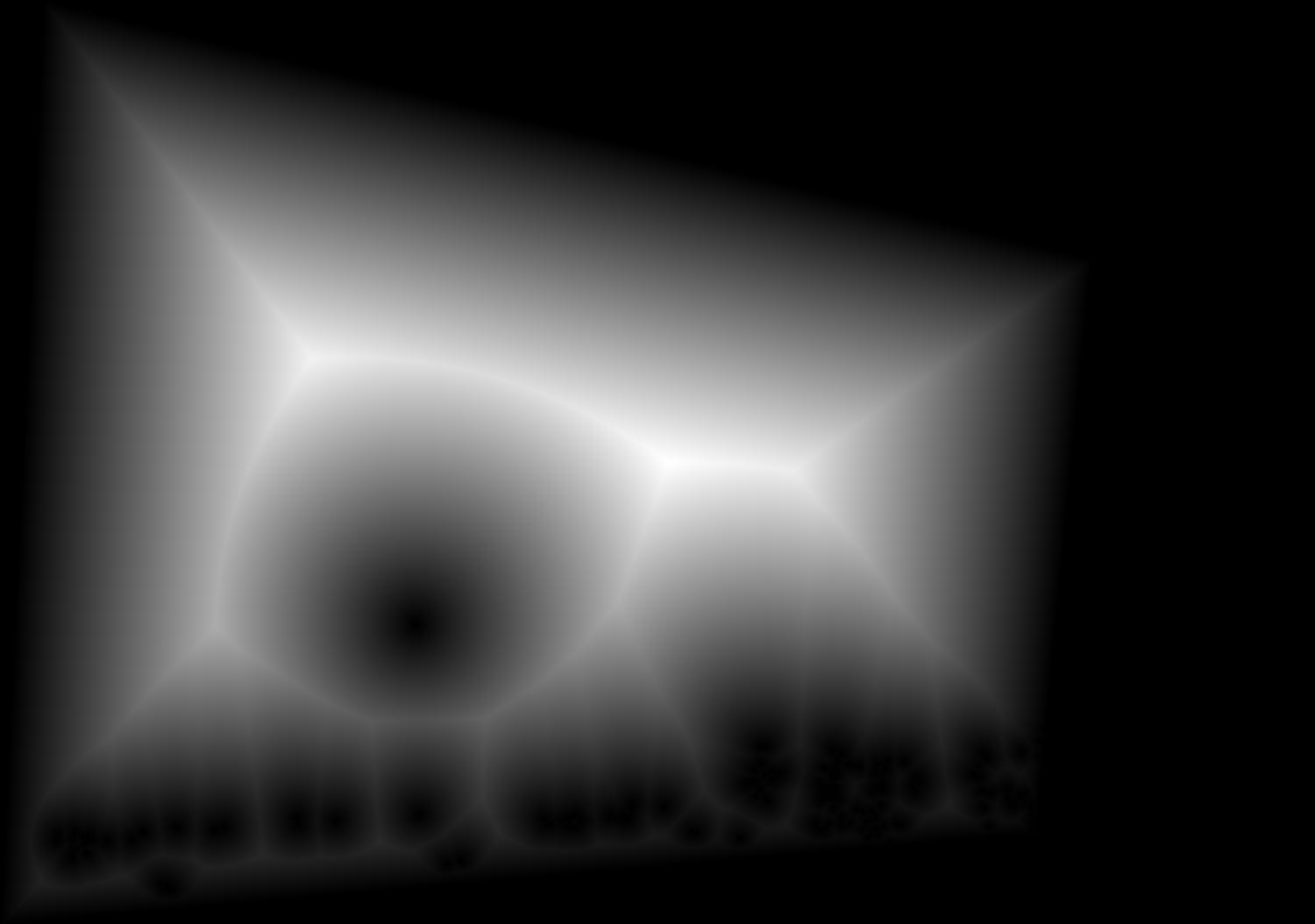
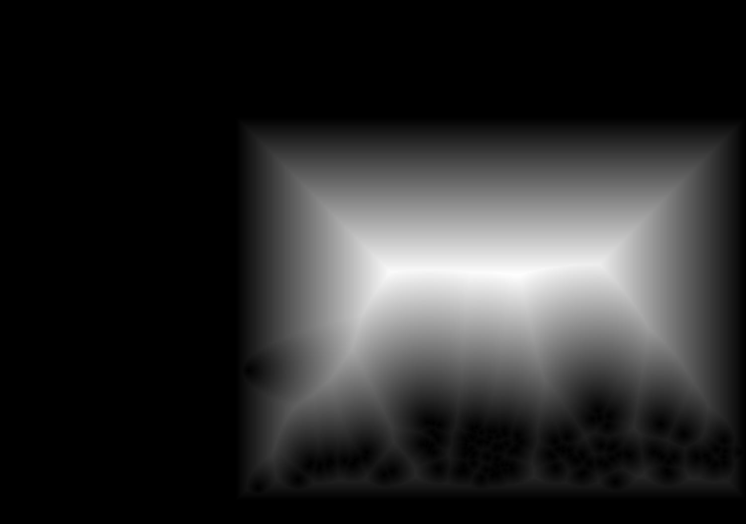
To blend the images, I used the two-band blending method from lecture. To reduce the presence of seams and ghosting, I used scipy.ndimage.distance_transform_edt to weight the mask pixel values relative to how far they were from the borders. I originally tried using the cv2.distanceTransform function but debugging that became really annoying due to it's lack of useful error messages. The reason why the borders of the images will produce seams is because during the gaussian blurring process, the blur kernel will take in black pixels from the edges, leading to a shading effect.

Here is the general flow for blending the two images together:

1. Compute the homography of the warped image to the reference image.
2. Compute the corners of the warped image and the reference image
3. Compute the size of the mosaic canvas
4. Compute the mask for the warped image and the reference image
5. Compute the distance transform for the mask
6. Find the low and high frequencies fo each image
7. Compute a weighted average of the low and high frequencies together using their masks.
8. Combine the low and high frequencies together
9. Blend the images together

Here is an example of what the distance transform mask looks like for my Chicago Skyline images in Part B.

Mask for Warped Image

Mask for Reference Image

Here are some example photos I took!

Sunset: The sunset image worked a lot better than I expected!

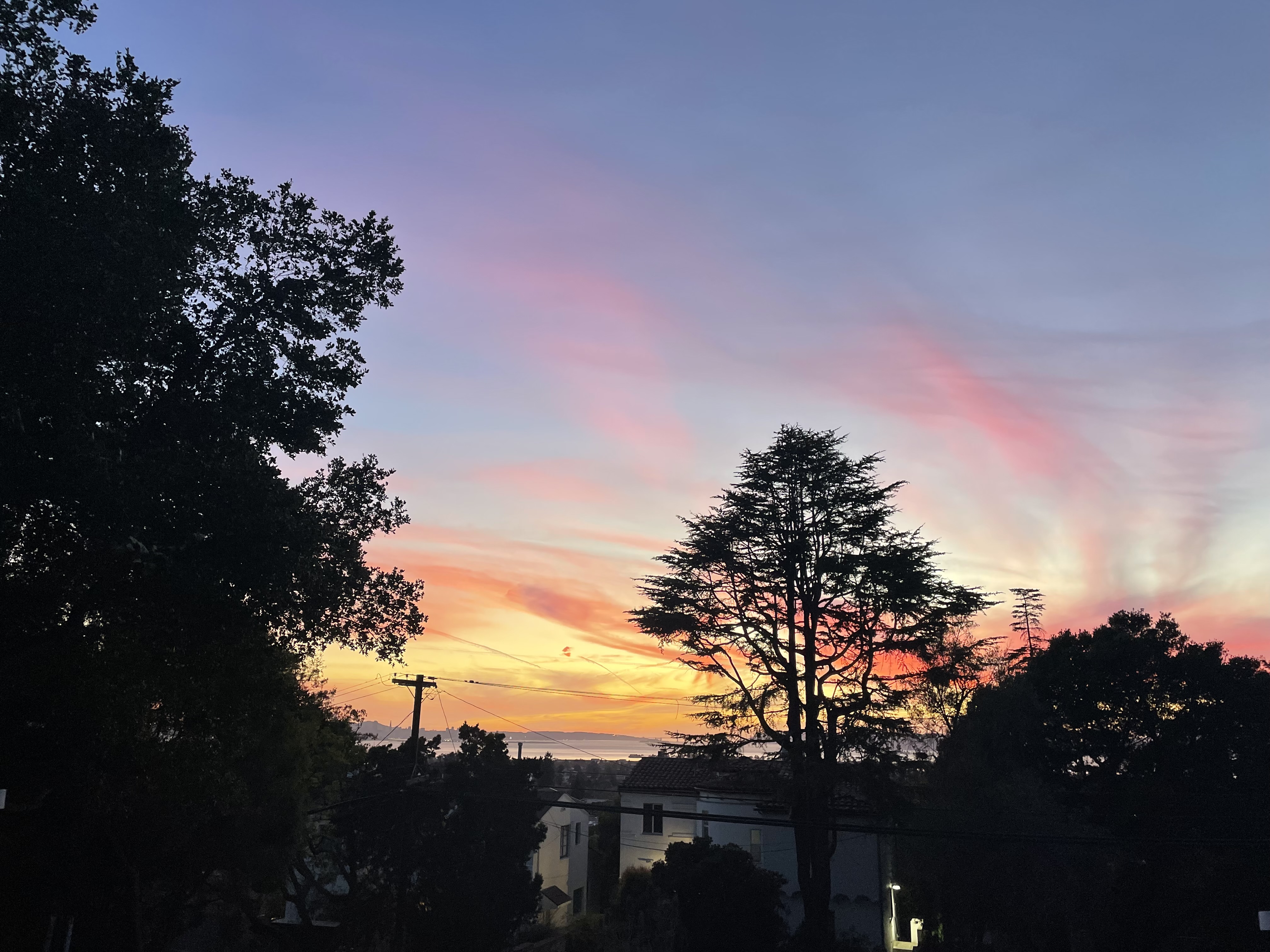
Sunset 1

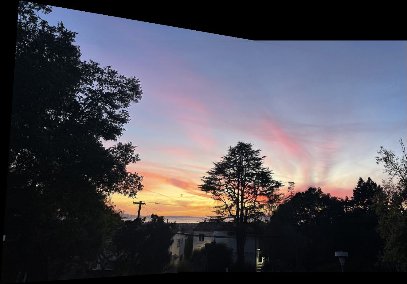
Sunset Mosaic

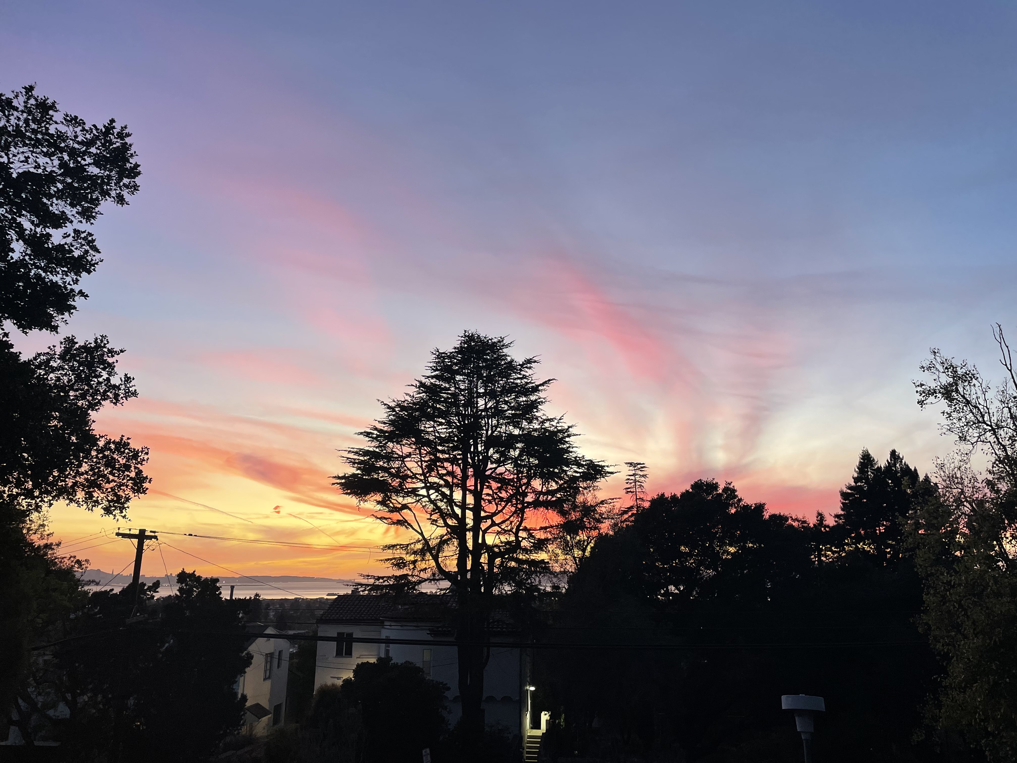
Sunset 2

Grass: Here, you can see a mild crease in the sky. It's not super obvious unless you squint, but I think that is something I can work on improving for Part B. Perhaps my blending is absorbing some of the border into the blend.

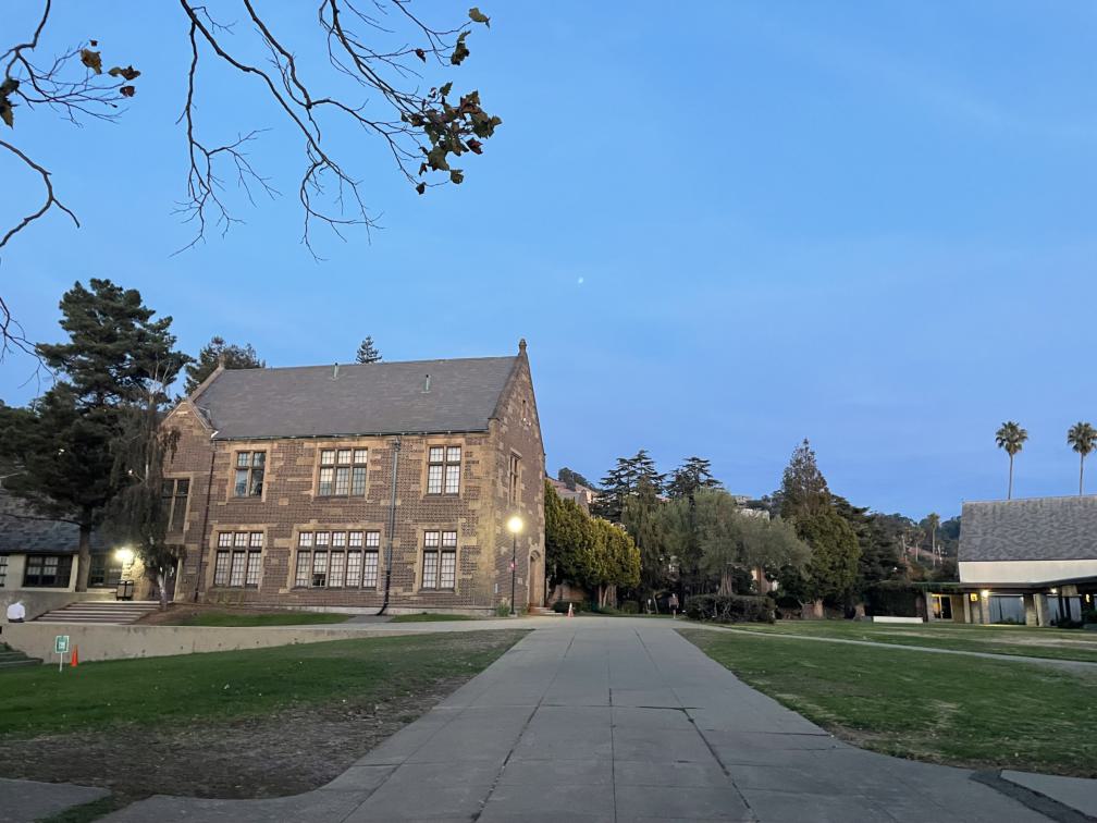
Pacific School of Religion 1

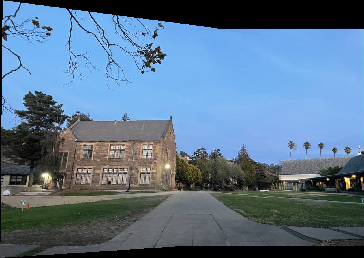
Pacific School of Religion Mosaic

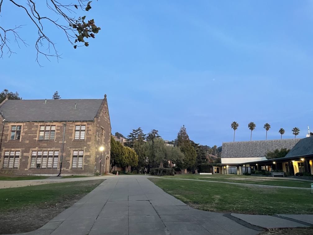
Pacific School of Religion 2

Philly: As you can see here, there is a little bit of blurriness at the bottom of the image, and the cars are mismatched. I believe this is because I was standing next to a busy street, so the cars naturally moved. Thus, in my second image, the cars shifted position! As we are limited by a 2D image, we cannot capture the cars in time.

Philly 1

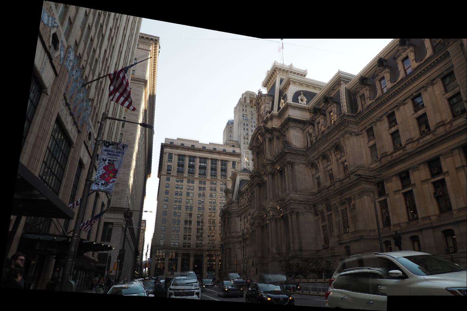
Philly Mosaic

Phlly 2

Feature-matching and Autostitching

For the second part of the project, we are using the methods outlined in Brown et al's paper “Multi-Image Matching using Multi-Scale Oriented Patches”, specifically sections 2, 3, 4, and 5. The goal of this section is we want to be able to automatically stich images into a mosaic since, as we learned in part a, choosing correspondance points is super tedious.

1. Detecting corners

For corner detection, I used the Harris Interest Point Detector in Section 2 of the paper. To identify the corners, I used the code in harris.py. I converted my image to grayscale and used get_harris_corners to retreive the harris score h and corners. The function returns the scores as (y, x) but I wanted to use the points in the form (x, y) so I transposed the returned array.

2. Extracting feature descriptors

For feature extraction, I followed Section 3's Adaptive Non-Maximal Suppression (ANMS) with c_robust = 0.9 (as recommended in the paper) and num_corners = 100.

To compute the actual ANMS score, followed the following procedure:

1. I obtained the scores of each corner by indexing h[corners[:, 0], corners[:, 1]].
2. Then, I computed the pairwise distances of the corners using the dist2 function provided in the harris.py starter code.
3. Next, I created a mask to determine if \( f(x_i) < c_{\text{robust}} \cdot f(x_j) \) by using array broadcasting scores[:, np.newaxis] < (c_robust * scores[np.newaxis, :]). This essentially compares the strength of each of the corners.
4. Applied the mask to my distance matrix of corner strength.
5. Set zero elements of the matrix to be infinity. This is useful since we perform a minimization operation in the next step. (If you forget to do this, you may end up with 0-1 cornerse and be very confused.)
6. To compute the minimum suppression radius, which minimizes the squared distances, I take np.min(masked_dists, axis=1), then obtain the sorted indices based on suppression radius from largest to smallest using (-radii).argsort(). Then, I use that to obtain the sorted corners and select the first num_corners points as my ANMS points.

Below is an example of the result of the Harris points vs the ANMS points!

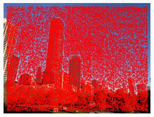
Harris Corners

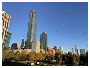
ANMS Corners

3. Extracting feature descriptors

To extract feature descriptors, I followed Section 4 of the paper. For every point in the ANMS points, I:

1. Extracted a 40x40 patch around the point.
2. Downsampled this patch to become 8x8.
3. Normalized the intensity by subtracting the mean and dividing by the standard deviation of the patch.
4. Flattened the patch to be (1, 192) using features.reshape(features.shape[0], -1)

Below are a sample of my features:

4. Matching feature descriptors

To match feature descriptors, Section 5 of the paper, I did the following:

1. Extracted the features and their corresponding points for both images.
2. For each feature compute the pairwise differences between the features of the the two images. I again used numpy array broadcasting (diff = features1[:, np.newaxis, :] - features2[np.newaxis, :, :]), which produces a (num_points, num_points, 192) matrix.
3. Take the squared differences and sum over all 192 pixels to get a 100x100 matrix of the sum of squared differences.
4. Sor each row (feature) from smallest to largest using np.sort(ssd).
5. The paper uses something called a Lowe Score, which is basically a comparison between the first nearest neighbor (NN) distance with the second NN distance. To do this, I computed lowe = nn_dists[:, 0] / nn_dists[:, 1] across all features.
6. Then, I created a mask lowe <= lowe_threshold so I could extract features lower than the Lowe score. This means that the feature is most closely matched with its 1NN. For my project, I used lowe_threshold = 0.3.
7. I obtained the indices of the 1NN for each feature ssd.argsort()[:,0], then create a list of the indices paired with their corresponding image 1 features via np.stack([np.arange(0, closest.shape[0]), closest]).T.
8. Finally, I filtered the index, feature pairs using matches[lowe_mask].

I used a lowe threshold of 0.3. Below are the first 12 match examples! The pictures are blurry because I'm blowing up an 8x8 image to be viewable on the screen.

Source Image

Destination Image

Source Image

Destination Image

5. Use a robust method (RANSAC) for homography

To implement RANSAC for computing homographies, I implemented the procedure we talked about in lecture, using these steps:

1. Using the matches obtained from Step 4 and the points from Step 2, I split my points into source and destination points matches_src, matches_dst = points1[matches[:, 0]], points2[matches[:, 1]].
2. Randomly select 4 points from the matches using np.random.choice(src_pts.shape[0], size=4,replace=False).
3. Compute the homography matrix using the 4 points using the computeH function from Part A.
4. Convert the source points to homogenous form (x, y, 1).
5. Transform source points into destination coordinates.
6. Unscale the transformed points, then remove the homogenous column.
7. Compute the number of inliers by computing the distance between the points and the homography matrix np.sqrt(np.sum((dst_pts - transformed_src) ** 2, axis=1)). Create a mask by checking if the distance is less than a threshold. If it is, then the point is an inliers.
8. Repeat steps 1-3 for steps iterations.
9. Throughout all iterations, keep track of the mask with the maximum number of inliers. At the end, use best_mask to return the source and destination points that produce the best homography. These are our corresponding points like in Part A.

I used a threshold of 0.8 and 1000 steps. Here are images of my final corresponding points (red points):

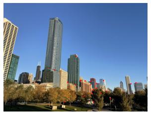
Source Image

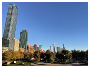
Destination Image

6. Final Mosaics

To create the final mosaics using auto-stitching, I used the best set of source and desination points from Step 5, computing the homography matrix using these points and blending them together like in Part A. Before I threw my points into homography, I had to remember to swap the x and y axes of my points due to the way they are stored. Here are some of my final mosaics!

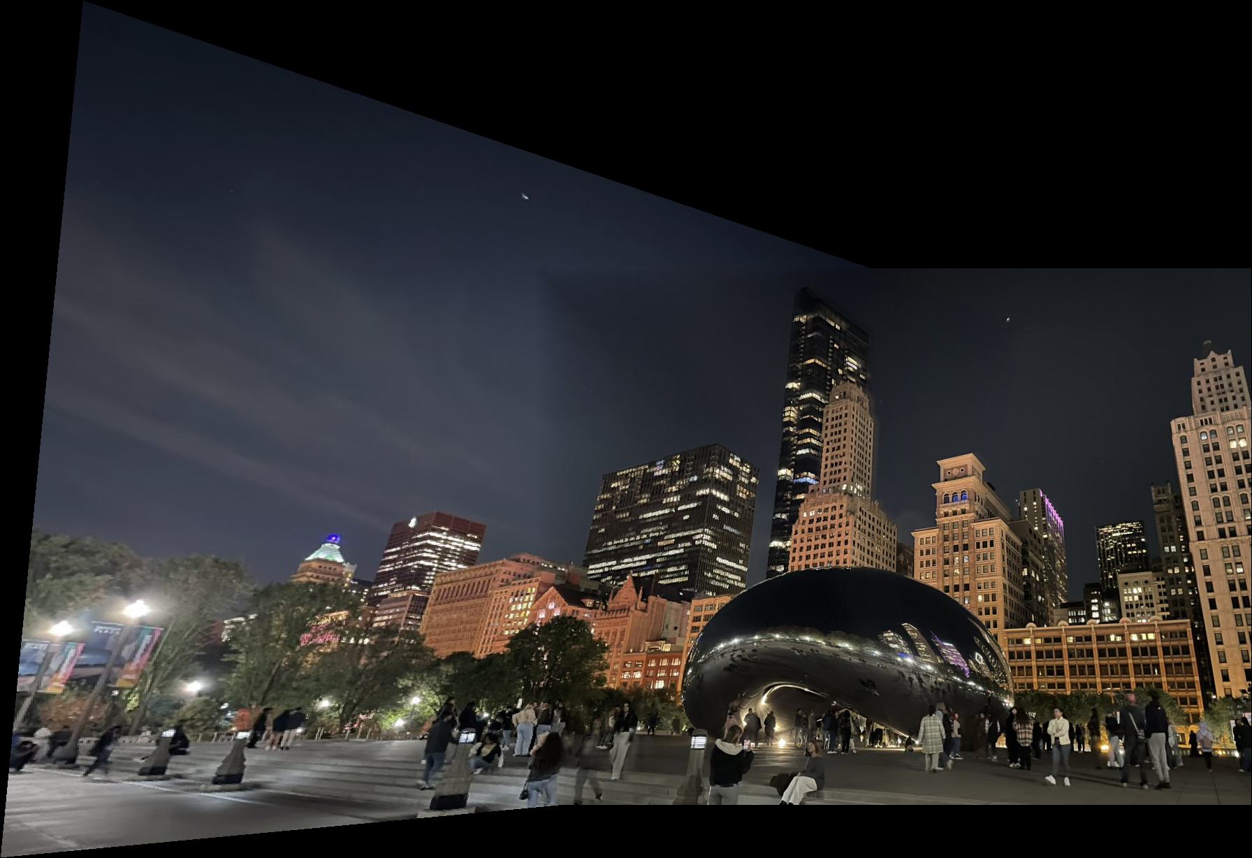
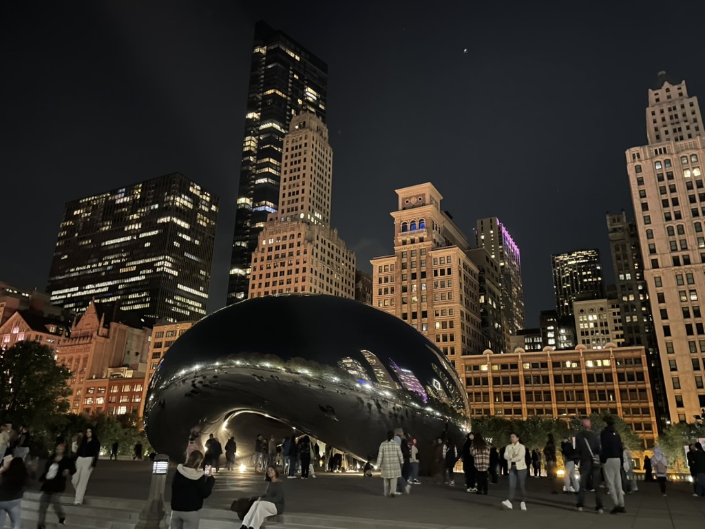
The Bean at Night

For this image, there is a bit of a seam in the middle since the exposure of the left image is different from the right image. This is due to iPhone's auto-exposure control. The result would look better once I implement some exposure correction.

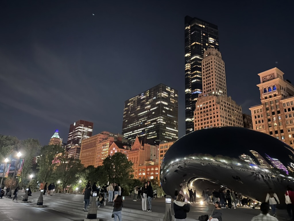
The Bean 1

The Bean Mosaic

The Bean 2

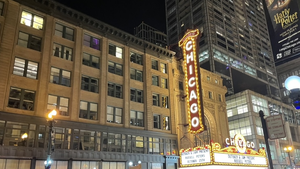
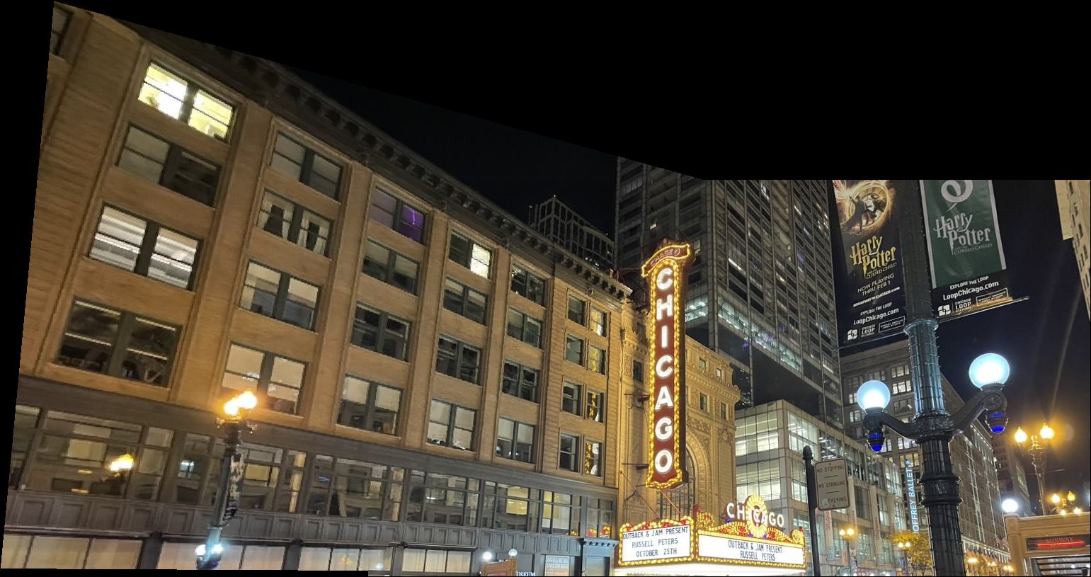
The Chicago Theater

For this image, I had to crop out the cars at the bottom of the image. The cars moved between the two frames, which made my auto feature detection match to the cars, yet the cars were in different positions in both photos so the mosaic alignment would not work properly.

The Chicago Theater 1

The Chicago Theater Mosaic

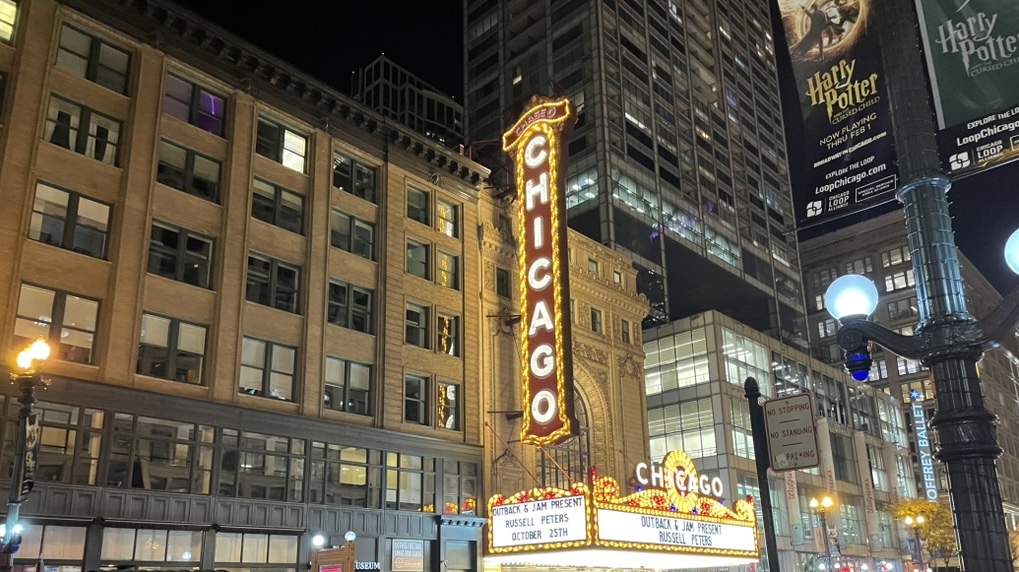
The Chicago Theater 2

Chicago Skyline

Here are photos I took during my last day in Chicago. It was on an early morning run near Lake Michigan!

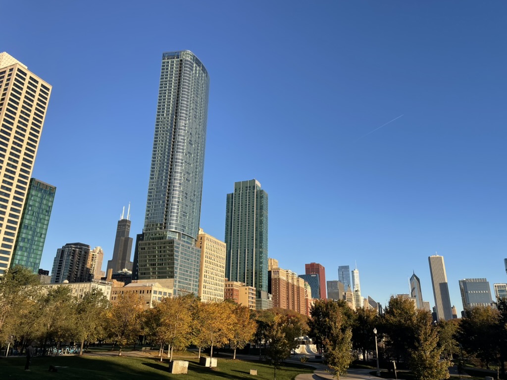
City 1

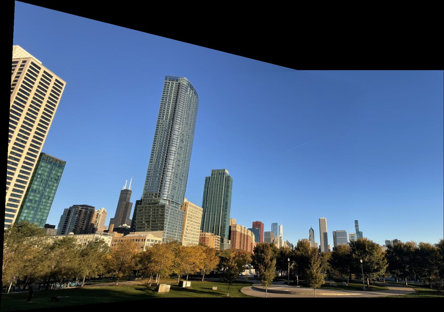
Chicago Skyline Mosaic

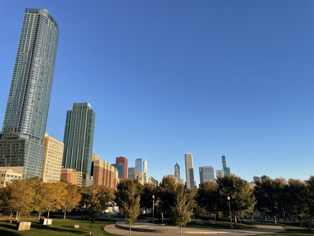
City 2

Reflection

I learned a lot in this project! It was really cool to see the history behind how panoramas are generated, and it gives me a greater appreciation for the work that has been put into the technology I use today. At first, I had trouble with my images due to mis-matched center of projections, but once I fixed those bugs, it was very exciting to see my mosaics come together. I previously worked with homographies in my research, but implementing it myself made me understand how they worked a lot more. I have new ideas on how to use homographies for rectifying a license plate collection that I have!

In Part B, what I found interesting was how the quality of your image greatly affects your auto-generated points. For example, I kept getting poorly stitched images only to realize that it was because I was capturing a dynamic scene. My algorithm was picking up corners that were moving. Thus, I was aligning to moving targets rather than stationary targets.