CS180: Introduction to Computer Vision & Computation Photography
Project 5
Fun With Diffusion Models!
Clara Hung
Project Overview
In this project, we work with diffusion models!!
Part 0: Setup / Sampling from the Model
Throughout this project, I use the random seed 11. Here are the three images generated from the starter code. Each of these is generated with 20 inference steps. Throughout this part of the project, we use DeepFloyd IF, a diffusion model trained by Stability AI.
First, I generated images from the model with the default 20 steps.
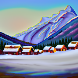
An oil painting of a snowy mountain village
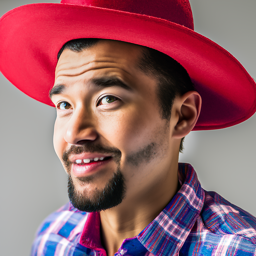
A man wearing a hat

A rocket ship
Here, I test increasing the number of inference steps to 100. The images contain more fine details than just using 20 steps. For example, the man photo has more distinct skin texture than the 20 step version. On the other hand, I think for simpler images, like the rocket, the 20 step version is better because it doesn't add extraneous details that make it look less realistic. The oil painting image had a similar quality. Oil paintings are known for their smooth, almost watercolor-like texture, and the 20 step version captures that well whereas the 100 step version is too precise.
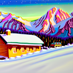
An oil painting of a snowy mountain village (100 steps)
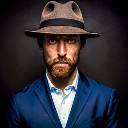
A man wearing a hat (100 steps)

A rocket ship (100 steps)
Next, I try only using 5 inference steps. Here, the images are much more abstract and blurry, almost reflecting a pointilist style of art. While the general structure of each image is still there, there are less realistic details than the 20 step version. For example, the rocket ship and the hat are not very recognizable.
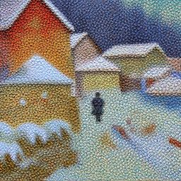
An oil painting of a snowy mountain village (5 steps)
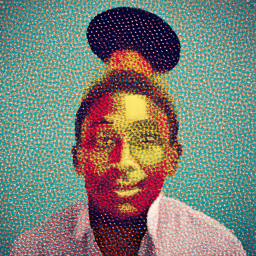
A man wearing a hat (5 steps)
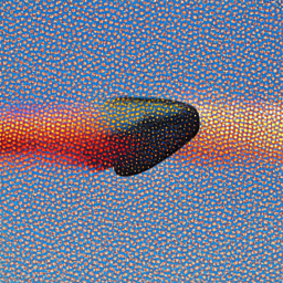
A rocket ship (5 steps)
Part 1: Sampling Loops
This section of the project involves writing our own sampling loops that use pretrained DeepFloyd denoisers. For many of these sections, we will be using the Campinile test image:
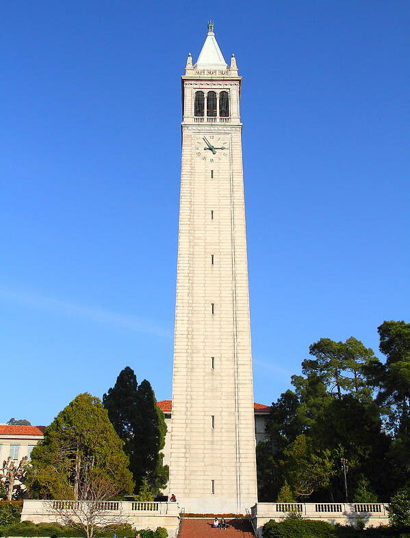
UC Berkeley's Campanile
1.1 Implementing the Forward Process
For the forward proess of a diffusion model, we take a clean image and add noies to it. The process is defined by computing:
$$x_t = \sqrt{\bar\alpha_t} x_0 + \sqrt{1 - \bar\alpha_t} \epsilon \quad \text{where}~ \epsilon \sim N(0, 1)$$
where \(x_0\) is the clean image and \(x_t\) is the noisy image at timestep \(t\) that we get from sampling from a Gaussian with mean \(\sqrt{\bar\alpha_t} x_0\) and variance \( (1- \bar\alpha_t)\). \(\bar\alpha_t\) is given and should be close to 1 for small t and close to 0 for large t.Test Image at the noise levels: 250, 500, 750

Forward Process with Noise Level 250

Forward Process with Noise Level 500

Forward Process with Noise Level 750
1.2 Classical Denoising
For each of the three noise levels in the previous part, I use a classical denoising model, e.g. gaussian blurring, to denoise the image. The results are as follows:

Classical Denoising at Noise Level 250

Classical Denoising at Noise Level 500

Classical Denoising at Noise Level 750
1.3 One-Step Denoising
For each of the three noise levels in the previous part, I use the DeepFloyd stage 1 model to denoise the image by estimating the noise and removing it. We can obtain the clean image by solving for \(x_0\) in terms of \(x_t\) using the equation above. Since this model was trained with text conditioning, we also use a text prompt embedding `"a high quality photo"`. The results are as follows:

One-Step Denoising at Noise Level 250

One-Step Denoising at Noise Level 500

One-Step Denoising at Noise Level 750
1.4 Iterative Denoising
The results from one-step denoising were better than classical denoising, but they could be better since you can see the image is still blurry. Thus, we use the following equation with strided timsteps to obtain our clean noise estimate:
\[ x_{t'} = \frac{\sqrt{\bar\alpha_{t'}}\beta_t}{1 - \bar\alpha_t} x_0 + \frac{\sqrt{\alpha_t}(1 - \bar\alpha_{t'})}{1 - \bar\alpha_t} x_t + v_\sigma \]Here are samples from different timesteps in the iterative denoising process:

Iterative Denoising at Timestep 690

Iterative Denoising at Timestep 540

Iterative Denoising at Timestep 390

Iterative Denoising at Timestep 240

Iterative Denoising at Timestep 90
Here is a comparison of the final results using different denoising methods.
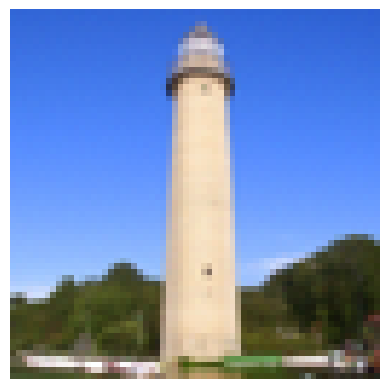
Final Result: Iterative Denoising

Final Result: One-Step Denoising

Final Result: Classical Denoising
1.5 Diffusion Model Sampling
So far, in the previous parts, we've only used the diffusion model to denoise an image. We can also generate images from scratch by sampling from the model. We are effectively denoising pure noise.
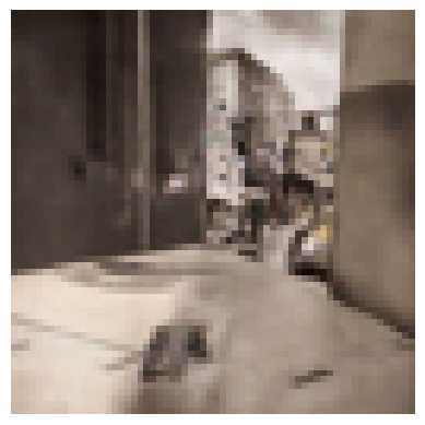
Generated Sample 1
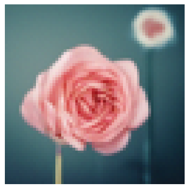
Generated Sample 2
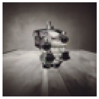
Generated Sample 3
Generated Sample 4
Generated Sample 5
1.6 Classifier-Free Guidance (CFG)
The generated images in the previous section are ok but not super high quality, and some of them don't make sense. Thus, to improve image quality, we use a technique called Classifier-Free Guidance (CFG) where we compute both a conditional and unconditional noise estimate \(\epsilon_c\) and \(\epsilon_u\). Our new estimate is now: \[\epsilon = \epsilon_u + \gamma (\epsilon_c - \epsilon_u)\] where \(\gamma\) controls the strength of the CFG. When \(\gamma = 0\), we get an unconditional noise estimate. When \(\gamma = 1\), we get a conditional noise estimate. Generally, we want to look at \(\gamma > 1\). Below are image samples from CFG. Noise how they are more high quality and realistic!
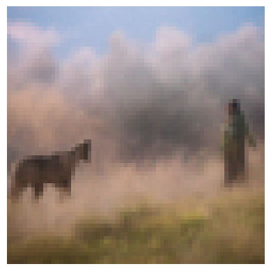
CFG Generated Image 1
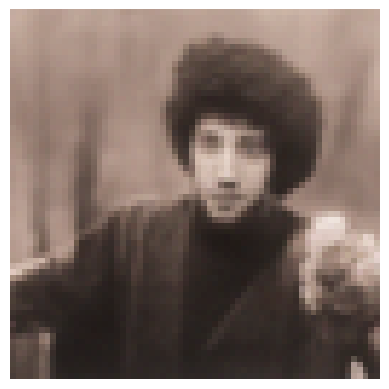
CFG Generated Image 2
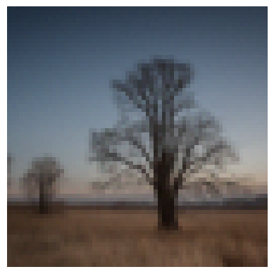
CFG Generated Image 3
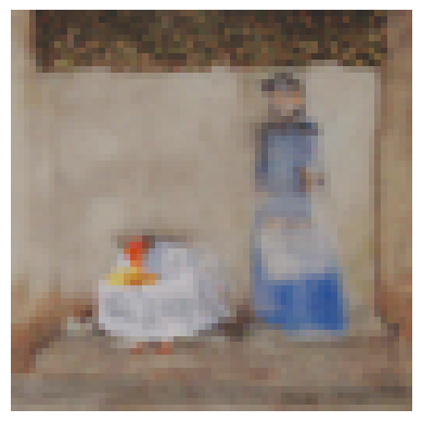
CFG Generated Image 4
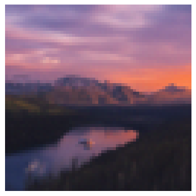
CFG Generated Image 5
1.7 Image-to-image Translation
Now, what we are going to do is to take the original test image, add a little bit of noise, then force it back to the original image wihtout any conditioning. At noise levels, we should get an image similar to the test image. Effectively, the model "edits" the image. Notice how we get increasingly closer to the test image! Recall our indices go from high to low noise levels.
Image Translation with Index 1
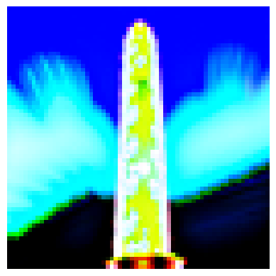
Image Translation with Index 3
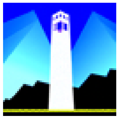
Image Translation with Index 5
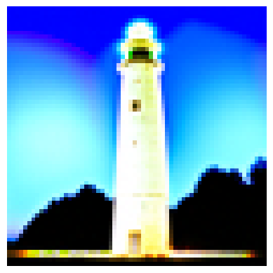
Image Translation with Index 7
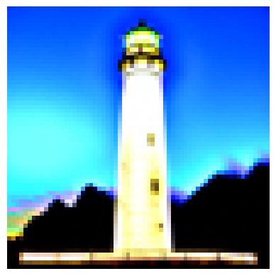
Image Translation with Index 10
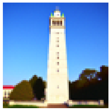
Image Translation with Index 20
1.7.1 Editing Hand-Drawn and Web Images
Another thing we can do is start with a nonrealistic image or some web image and project it onto the natural image manifold. The model will try to force the image into a more "realistic" looking image. Below, I tried with a web images and hand-drawn scribbles!
Web Image: I tried using a random image of bear clipart on the internet.

Original Clipart

Web Image Translation with Noise Level 1

Web Image Translation with Noise Level 3

Web Image Translation with Noise Level 5

Web Image Translation with Noise Level 7

Web Image Translation with Noise Level 10

Web Image Translation with Noise Level 20
Hand-Drawn Image #1: Here, I drew an image of a simple looking sprout. Notice how the model thinks it looks like a bird, which I can see.

Original Clipart

Hand-Drawn Image 1 with Noise Level 1

Hand-Drawn Image 1 with Noise Level 3

Hand-Drawn Image 1 with Noise Level 5

Hand-Drawn Image 1 with Noise Level 7

Hand-Drawn Image 1 with Noise Level 10

Hand-Drawn Image 1 with Noise Level 20
Hand-Drawn Image #2: here, I tried drawing an image of a coffee mug. The model thinks it looks like a lady with dark hair.

Original Clipart

Hand-Drawn Image 2 with Noise Level 1

Hand-Drawn Image 2 with Noise Level 3

Hand-Drawn Image 2 with Noise Level 5

Hand-Drawn Image 2 with Noise Level 7

Hand-Drawn Image 2 with Noise Level 10

Hand-Drawn Image 2 with Noise Level 20
1.7.2 Inpainting
The same procedure can be used to implement in-painting, where we choose a mask and ask the model to fill in the image, leaving everything inside the mask alone but replace everything outside the edit.
Below is an example of the image, mask, and area to replace. This was the only sample where I actually saved the intermediate outputs (RIP), but please trust me on this! I created three sample inpaintings below.

Image

Mask

To Replace

Test Image Result

Bear Result

Tree Result
1.7.3 Text-Conditional Image-to-image Translation
Next, we will do a similar thing but guide the projection onto the manifold of images using a text prompt to control that projection. The image should gradually look more like the original image but also like the text prompt.
Example 1: Test Image with Rocket Embedding

Noise Level 1

Noise Level 3

Noise Level 5

Noise Level 7

Noise Level 10

Noise Level 20
Example 2: Green plains with waterfall embedding

Noise Level 1

Noise Level 3

Noise Level 5

Noise Level 7

Noise Level 10

Noise Level 20
Example 3: Bear with Dog Embedding

Noise Level 1

Noise Level 3

Noise Level 5

Noise Level 7

Noise Level 10

Noise Level 20
1.8 Visual Anagrams
Now, we can build off of everything we've learned so far to implement Visual Anagrams to create optical illusions with diffusion models. We can create images that look like something in one orientation but something else in another orientation by computing the noise of each embedding, with one right-side-up and one upside-down. Then we average the two noise estimates. Mathematically, it looks like: \[\epsilon_2 = \text{flip}(\text{UNet}(\text{flip}(x_t), t, p_2))\] \[\epsilon_2 = \text{flip}(\text{UNet}(\text{flip}(x_t), t, p_2))\] \[\epsilon = (\epsilon_1 + \epsilon_2) / 2\]
Visual Anagram #1:
- Upright: "an oil painting of people around a campfire"
- Upside-down: "an oil painting of an old man"
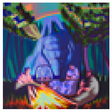
An Oil Painting of People Around a Campfire (Upright View)

An Oil Painting of an Old Man (Inverted View)
Visual Anagram #2:
- Upright: "a coastal village with boats"
- Upside-down: "a mountain landscape with trees"
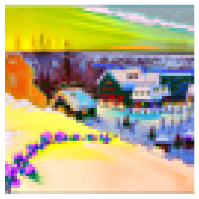
A Coastal Village with Boats (Upright View)

A Mountain Landscape with Trees (Inverted View)
Visual Anagram #3:
- Upright: "a lithograph of waterfalls"
- Upside-down: "an oil painting of a snowy mountain village"
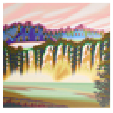
Caption for upright image

Caption for upside-down image
1.9 Hybrid Images
We're almost at the end!! Finally! We can implement Factorized Diffusion to create hybrid frequency images just like we did in Project 2! To create a hybrid image, we use a similar process as 1.8 but rather than averaging, we pass the noise estimate of one prompt emebedding through a low-pass filter and another through a high-pass filter so we can see different images at close and far distances. Below are my examples! For the final one, you can see that there is a dog in the nature.

Hybrid image of a skull and waterfall. LF: Skull; HF: Waterfall

Hybrid image of a pencil and rocket. LF: Rocket; HF: Pencil

Hybrid image of a dog and a waterfall. LF: Waterfall; HF: Dog
Part 1: Training a Single-Step Denoiser
In this part, we train our own diffusion model on MNIST. Our goal is to train a denoiser \(D_{\theta}\) such that it maps a noisy image \(z\) to a clean image \(x\). We do this by optimizing over the L2 Loss: \[L = \mathbb{E}_{z,x} \|D_{\theta}(z) - x\|^2\] We train our denoiser by generating data pairs of \((z, x)\) For the training batch, we can generate our noisy image from our clean image using the noising process: \[z = x + \sigma \epsilon,\quad \text{where }\epsilon \sim N(0, I)\]
Below are visualizations of the noising process over \(\sigma = [0.0, 0.2, 0.4, 0.5, 0.6, 0.8, 1.0]\)
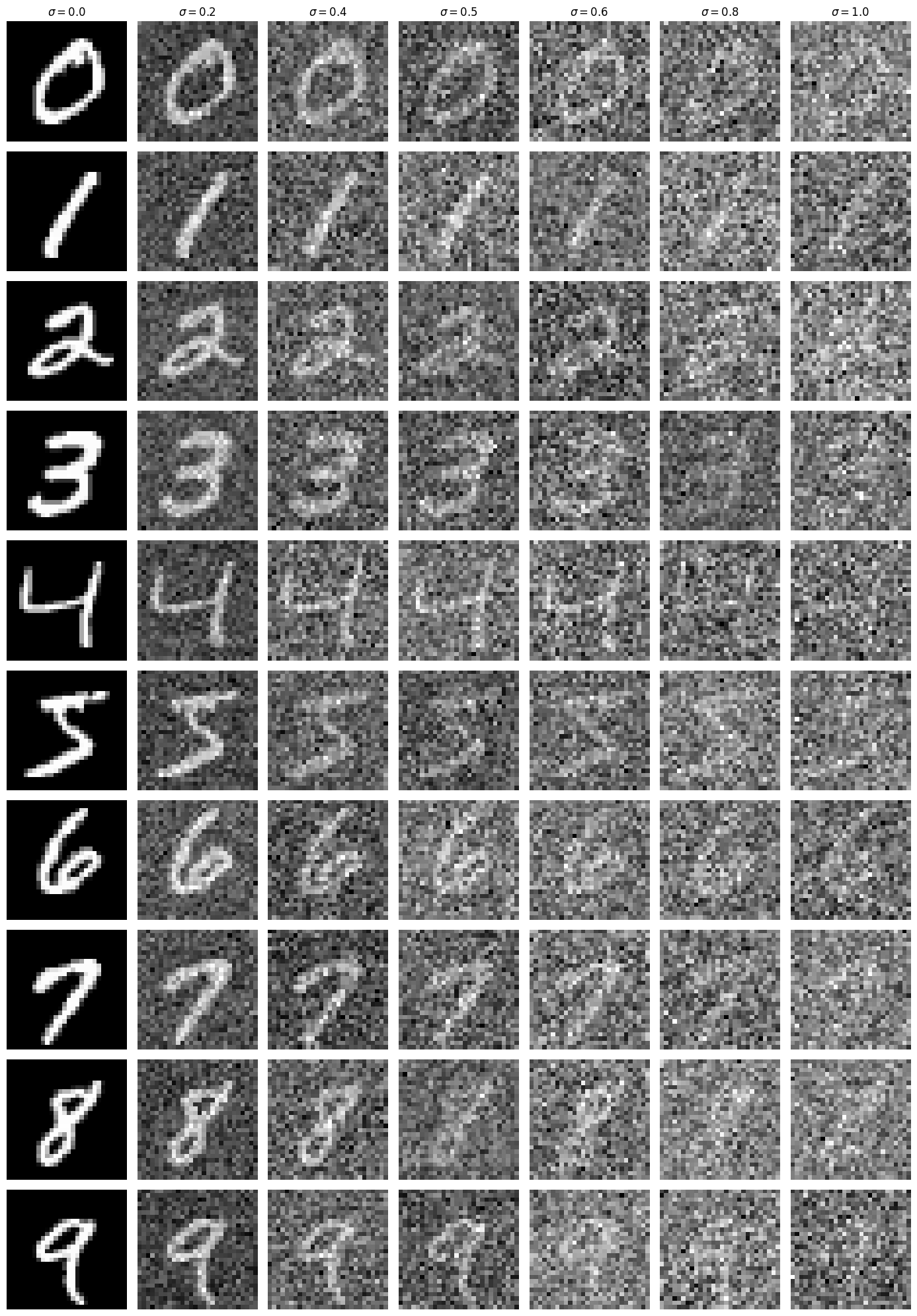
Visualization of the noise process
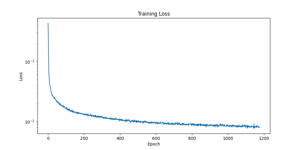
Log-scale loss curve of UNET training
Here are visualizations of my results after the 1st and 5th epochs. Notice how more epochs lead to better looking results. In these results, I randomly picked digits, but in retrospect, it probably would have been better to choose the same digits to visualise. To be fair, the speci did not specify that I should choose the same digits, so oh wells, I'm kind of tired of UNETs.
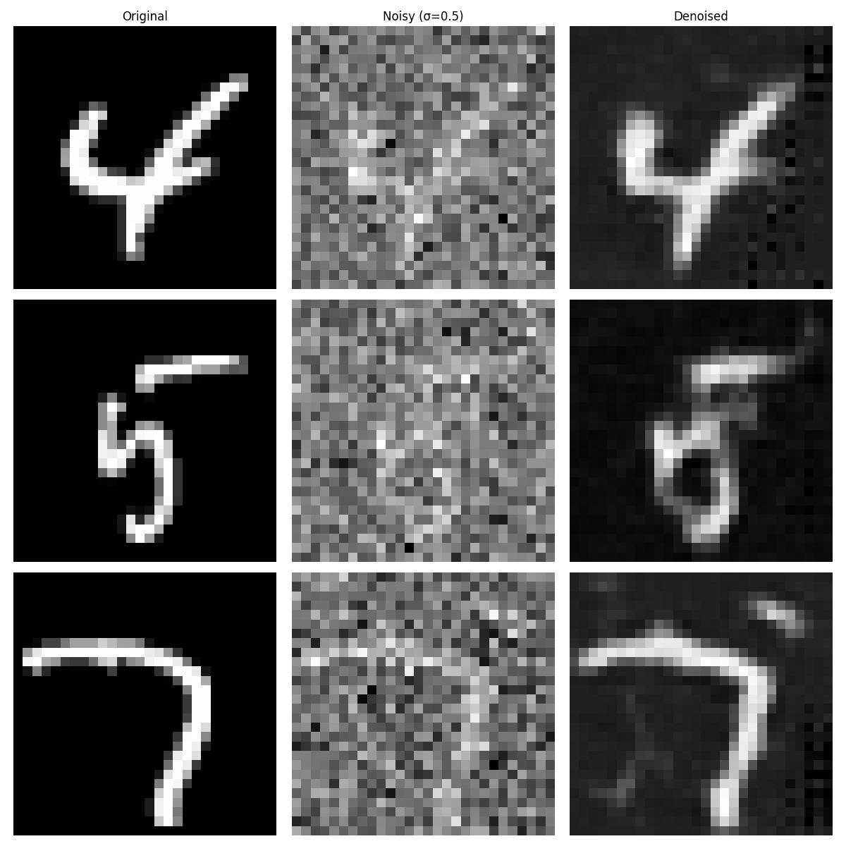
Results after Epoch 1
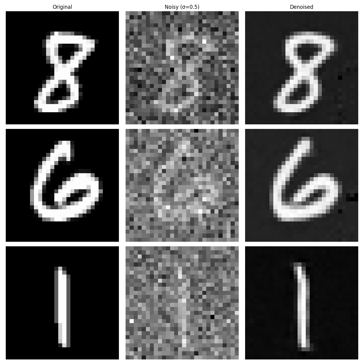
Results after Epoch 5
One other test we can do is to test on out of distribution images. Our denoiser was trained on MNIST digist noised with \(\sigma = 0.5\), but what happens to the denoiser on different sigmas that it wasn't trained for? Below is an example of the UNET performance on varying levels of sigma. Notice that performance is best for noise levels less than 0.5.

Out of Distribution Test Result
Part 2: Training a Diffusion Model
Can you believe it? The end is near!! Now, we are ready to train a UNET model to iteratively denoise an image. We will use DDPM in this part. Rather than denoising the image directly, we will train a UNET to estimate the noise in the image. Then, we can use the DDPM equations like we did in Part A to remove the moise from the image. We noise the image according to: \[x_t = \sqrt{\bar\alpha_t} x_0 + \sqrt{1 - \bar\alpha_t} \epsilon \quad \text{where}~ \epsilon \sim N(0, 1).\]
While we could train separate UNETs for each time-step we are after, it is much easier for us to train a single UNET conditioned on a given timestep, giving us a final objective function of: \[L = \mathbb{E}_{z,x} \|\epsilon_{\theta}(z, t) - \epsilon\|^2\]
For this process, we define a list of \(\alpha, \bar\alpha, \beta\) values with \(T = 300\), batch size 128, hidden dimensions 64, the Adam optimizer with an initial LR of 1e-3, an exponential LR decay scheduler with gamma of \(0.1^{(1.0 / \text{num_epochs})}\). We train for 20 epoch since this is a more difficult task than the previous part.
Here is a plot of my loss over the training process:
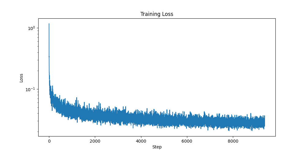
Log-scale loss curve of Time-Conditioned Training/p>
We can also sample from the UNET using a process similar to sampling in part A. For this sampling loop, we implement the DDPM equations. Below are some samples across different epochs. You can see that the digits don't look great, but their quality improves across epochs.
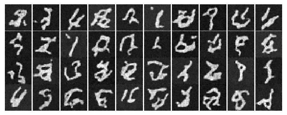
Results after Epoch 1
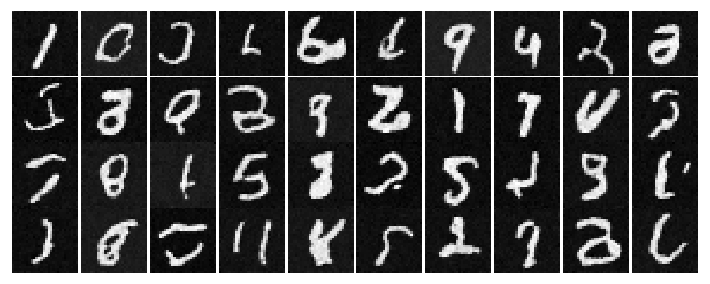
Results after Epoch 5
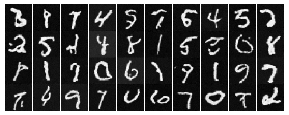
Results after Epoch 10
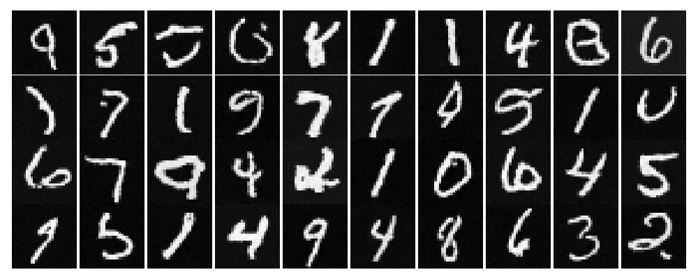
Results after Epoch 15
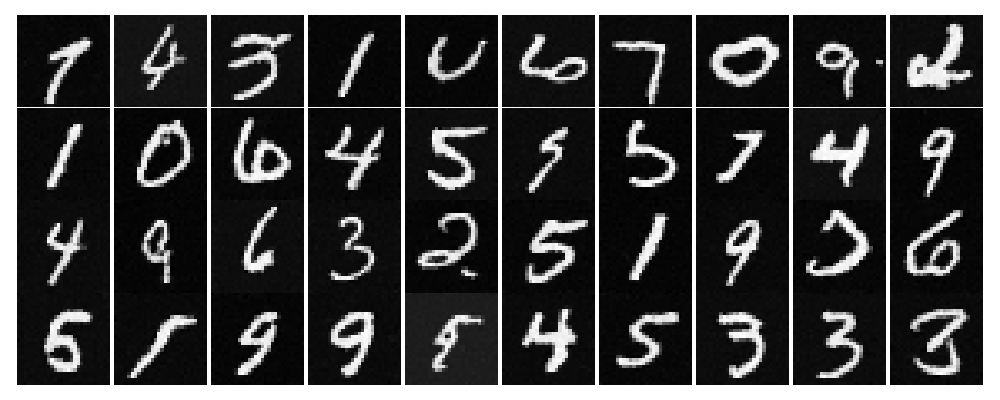
Results after Epoch 20
How can we fix these digits? Recall, perhaps from 189, that we can greatly improve our results if we add class-conditioning since each digit has its unique characteristics that can be learned a whole lot easier if we ask the UNET to condition on the class. Like we noticied in part A, for class-conditioning, we have to add CFG for the results to be good. For class-conditioned networks, we have to slightly tweak our network by adding a one-hot vector for our classes, which are the digits from 0-9. Additionally, we add a 10% dropout for the class vector by setting it to zero 10% of the time. Now, our UNET is conditioned on both time and class. For training, we use the same hyperparameters and LR scheduler as in the time-conditioned model. Below is my loss curve for training:
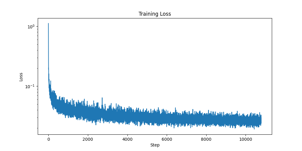
Log-scale loss curve of Time-Conditioned Training with CFG
Below are some samples across different epochs, where I draw 4 instances of each digits. You can see that the digits look much better than before. The quality of the digits improves across epochs as the shape becomes more defined and the strokes become slightly thinner and less like a toddler drew it..
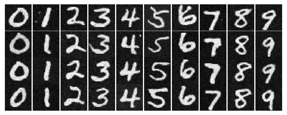
Results after Epoch 1
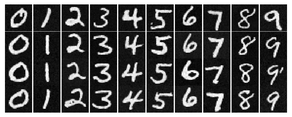
Results after Epoch 5
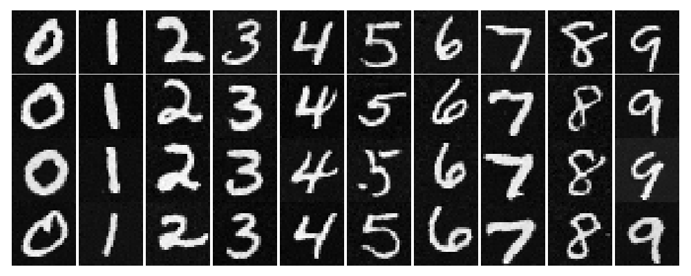
Results after Epoch 10
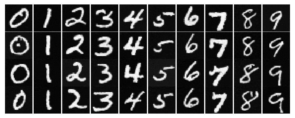
Results after Epoch 15
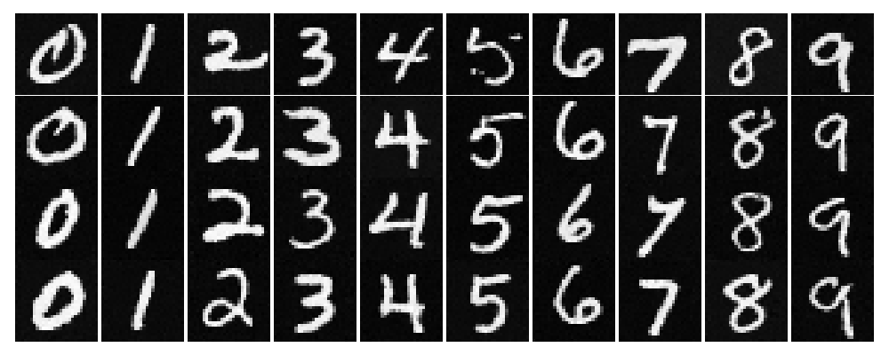
Results after Epoch 20